An Automatic Prover for the Elementary Functions - University of

MetiTarski: An Automatic Prover for the Elementary Functions Behzad Akbarpour and Lawrence C. Paulson Computer Laboratory, University of Cambridge, England {ba265,lcp}@cl.cam.ac.uk

Abstract. Many inequalities involving the functions ln, exp, sin, cos, etc., can be proved automatically by MetiTarski: a resolution theorem prover (Metis) modified to call a decision procedure (QEPCAD) for the theory of real closed fields. The decision procedure simplifies clauses by deleting literals that are inconsistent with other algebraic facts, while deleting as redundant clauses that follow algebraically from other clauses. MetiTarski includes special code to simplify arithmetic expressions.

1

Introduction

Many branches of mathematics, engineering and science require reasoning about the elementary functions: logarithms, sines, cosines and so forth. Few techniques are known for automatically proving statements involving such functions. We have been working on an approach that involves replacing functions by polynomial upper or lower bounds, attempting to reduce the problem to the theory of real closed fields (RCF), and then applying a suitable decision procedure. The theory of real closed fields (RCF) concerns equalities and inequalities involving addition, subtraction and multiplication. (We call logical formulas in this theory algebraic.) Real closed means every positive number has a square root. The decision procedure works by eliminating quantifiers from the supplied formula; for example, ∃x. ax2 + bx + c = 0 reduces to (a 6= 0 ∧ b2 − 4ac ≥ 0) ∨ (a = 0 ∧ b 6= 0) ∨ (a = b = c = 0). Both universal and existential quantifiers can be eliminated, but our current experiments involve refuting purely existential formulas. Tarski proved the decidability of RCF in the 1930s, but his procedure was impractical [10]. McLaughlin and Harrison [17] recently implemented a more efficient procedure credited to H¨ormander [13] and Cohen. We used it in earlier work [1, 2], but unfortunately it fails to terminate if applied to a polynomial of degree greater than six. QEPCAD-B [6, 12] is an advanced implementation of cylindrical algebraic decomposition (CAD), which is the best available decision procedure for the complete theory of RCF [10]. CAD is still doubly exponential in the number of variables, but it is polynomial in other parameters such as size of the input. In our experience, QEPCAD usually returns quickly. Its main drawback is that we have to run it as a separate process, while Harrison’s ML code could be integrated with that of Metis.

Our approach to proving inequalities involving elementary functions is to replace function occurrences one by one with appropriate upper or lower bounds. Once we have also eliminated occurrences of division, we can call QEPCAD. Daumas et al. [9] present families of upper and lower bounds for square roots, trigonometric functions, logarithms and exponentials. The approach can obviously be generalized to handle a wide variety of well-behaved functions. Our approach requires a full theorem prover even to prove simple inequalities. The bounds typically have side conditions that must be proved. Case analysis is necessary when eliminating division and often when substituting bounds. We chose to modify a resolution theorem prover, rather than implementing a theorem prover from scratch. Impressive examples of the latter approach include Analytica [8] and Weierstrass [5]. However, we felt that writing an entire prover would require more effort than modifying a resolution prover, while delivering inferior results. We were also inspired by SPASS+T [18], which effectively combines the resolution theorem prover SPASS with various SMT solvers. For the resolution prover, we chose Joe Hurd’s Metis [14]. Compared with leading provers, it is slow (being coded in Standard ML rather than C) and it lacks many refinements (such as advanced data structures for indexing). However, it implements the superposition calculus [4] and its code is extremely clear. Paper outline. We begin by describing (§2) how we modified the resolution prover Metis. We then discuss (§3) the upper and lower bounds we use. We present a table of new results (§4) along with brief conclusions (§5).

2

Modifications to the Resolution Prover

In order to make this paper self contained, we briefly outline the general approach, which was described in our previous paper [1].

Contradiction found

Passive clause set

selected clause

new clauses

inference rules

simplification

deduced clauses

Active clause set

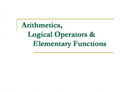
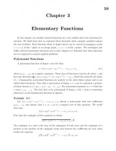
Fig. 1. The main loop of resolution

A resolution prover accepts its problems in conjunctive normal form. Seeking a contradiction, the conjecture to be proved is negated and conjoined with any

axioms. The entire problem is then transformed into a conjunction of disjunctions. Each disjunction is called a clause. Each member of a disjunction is an atomic formula or its negation, and is called a literal. Each resolution inference combines two clauses and yields new clauses. If the empty clause emerges, the proof is finished because the desired contradiction has been found. A resolution prover’s main loop (Fig. 1) manages two sets of clauses, Active and Passive [16]. At the start, all clauses belong to Passive. At each iteration, a Passive clause is selected and moved to Active. New clauses are inferred by resolving this clause with each of the other Active clauses. The new clauses are simplified and then added to Passive. MetiTarski is a version of the Metis prover modified in several respects: – Its implementation of the Knuth-Bendix ordering supports subterm coefficients [15]. This encourages the replacement of functions by bounds, even if the bounds superficially appear to be more complex. – The integer constants are available. Note that all variables are assumed to range over the real numbers. – A list of all ground algebraic clauses is maintained. They may contain only constants (including Skolem constants) and the functions +, − and ×. – Arithmetic expressions are simplified in order to identify redundant forms and to isolate the elementary functions. – Ground algebraic literals that are inconsistent with existing algebraic facts are deleted from every new clause. This brings us closer to the empty clause. – New clauses in that follow in RCF from existing algebraic facts are regarded as redundant and deleted. This reduces the use of space and time. 2.1

Arithmetic Simplification

MetiTarski uses a sparse recursive representation of polynomials. Originally, our sole objective was to map all variants of an expression to a unique canonical form [1]. We have added the objective of supporting the proof search by identifying occurrences of division and functions. Horner normal form. The idea behind our representation is that any polynomial in x can be rewritten in recursive form as p(x) = an xn + · · · + a1 x + a0 = a0 + x(a1 + x(a2 + · · · x(an−1 + xan )). We can express a multivariate polynomial as a polynomial in one variable whose coefficients are polynomials in other variables. For example, we can represent the polynomial 3xy 2 + 2x2 yz + zx + 3yz as [y(z3)] + x([z1 + y(y3)] + x[y(z2)]), where the terms in square brackets are considered as coefficients.

The Treatment of Division. Our normal form supports the operations of addition, subtraction, and multiplication. Division by an integer (or a rational number) does not present a problem, since a coefficient can be a rational number: the divisor is recursively supplied to the normal form conversion. General nested divisions can occur in expressions as a proof develops. Without special treatment, they will be difficult to eliminate and the RCF decision procedure will not be applicable. We transform an expression containing division into a rational function according to the following rules. (We identify E with E1 if necessary.) x2 x1 y2 + x2 y1 x1 + = y1 y2 y1 y2 x1 x2 x1 y2 − x2 y1 − = y1 y2 y1 y2

x1 x2 x1 x2 × = y1 y2 y1 y2 x1 x2 x1 y2 ÷ = y1 y2 y1 x2

The effect is to replace nested divisions by one single division, which as the outermost symbol can be eliminated by one proof step using an appropriate division axiom. In this example, three divisions are replaced by one.   x x2 1
= 1 2 y y(x + 1) x+ x We add literals to the resulting clause to account for the possibility of division by zero. In particular, if we simplify x1 /y1 + x2 /y2 then we make the resulting clause conditional on y1 6= 0 and y2 6= 0. However, for (x1 /y1 ) × (x2 /y2 ) and (x1 /y1 ) ÷ (x2 /y2 ), no such conditions are necessary. That is because we define x/0 = 0. It is trivial to see that (x1 /y1 )(x2 /y2 ) = 0 if and only if any of x1 , x2 , y1 , y2 , are zero, and in this they agree with the corresponding right-hand side. The alternative of introducing an error value and defining x/0 = ∞ would introduce great complications.1 Isolating Function Occurrences. We attempt to restore inequalities to a natural form. For example, we simplify X ≤ Y by normalizing X − Y , yielding an equivalent form X 0 ≤ Y 0 where X 0 and Y 0 both have positive coefficients. We have strengthened this process to isolate occurrences of elementary functions. In the Horner normal form transformation, we regard any non-algebraic term (typically a function occurrence) as a variable. We order the variables, taken in this general sense, using Metis’s built-in Knuth-Bendix ordering. This ensures that one of the function occurrences will appear as the outermost “variable.” If we detect this situation, we leave this term by itself on one side of the inequality, for example as ln(t) ≤ u. We even divide both sides by any constant coefficient, but at present we have no way of isolating the function in cases such as x ln(t) ≤ u. This challenge is a focus of our current work. 1

Harrison [11, §2.5] discusses various approaches to formalizing “undefined”, taking 1/0 = 0 as an example.

2.2

Algebraic Literal Deletion

Literal deletion [1] simplifies new clauses that emerge from inference rules. For each ground algebraic literal in such a clause, we conjoin it with the negations of all ground algebraic literals in that clause (its context) and with all ground algebraic clauses known to the prover. We then form the existential closure of this formula, taking as variables all Skolem constants present in that formula. If the RCF solver (QEPCAD) reduces this formula to false, then that literal is deleted. This is the primary mechanism by which the decision procedure contributes to deduction. As a small example, suppose we are trying to prove ∀x. − 3 < x < 1 → ln(1 − x) ≤ −x with the help of a range-restricted polynomial upper bound f2 , ∀x. 2 ≤ x ≤ 4 → ln(x) ≤ f2 (x). Skolemization of the conjecture will yield three clauses, with u a Skolem constant: −3 < u

u 1 − u ∨ 1 − u > 4. Ordinary arithmetic simplification can reduce 2 > 1−u to u > −1, and 1−u > 4 to −3 > u, but if f2 (1 − u) is a complicated polynomial, then only QEPCAD can achieve a real simplification: we give it the formula ∃u. f2 (1 − u) ≤ −u ∧ u ≤ −1 ∧ −3 ≤ u ∧ −3 < u ∧ u < 1 . {z } {z } | | negated literals

algebraic clauses

Provided f2 is a sufficiently tight bound, the result will be false and the literal can be deleted. The literal u < −1 turns out to be consistent with its context. Then we call QEPCAD for −3 > u: ∃u. −3 > u ∧ u ≤ −1 ∧ −3 < u ∧ u < 1. This again is false, and the final simplified clause is u > −1. It is a ground algebraic clause and will be added to our list. We have tightened the range of u to −1 < u < 1; if it becomes empty, then we have reached a contradiction. In this example, the constraints that accumulate are essentially linear. More generally, the use of rational function upper and lower bounds causes an accumulation of algebraic constraints, which eventually turn out to be inconsistent.

2.3

Algebraic Subsumption

Resolution theorem provers generate many redundant clauses. To conserve space, they typically delete any clause that is a syntactic instance of another. We generalize this redundancy criterion, known as subsumption, by performing an analogous redundancy check in the RCF theory. When a new clause is generated, we identify its ground algebraic literals and form their disjunction. If this disjunction is an algebraic consequence of existing algebraic facts, then we ignore the clause. Thus the formulas given to QEPCAD do not contain redundant conjuncts. This technique can even improve the performance of some failing proofs so that they fail finitely rather than running forever. The resulting performance improvement depends on other aspects of the formalization; at present only four percent of our problems are proved significantly faster when this technique is enabled. Recall our previous example, where the ground algebraic clauses included −1 < u and u < 1. Suppose that a resolution step yields the following clause: ln(1 − u) ≤ u2 ∨ u2 < 2 ∨ 4u > 3. Algebraic subsumption will call QEPCAD with the formula ∃u. u2 ≥ 2 ∧ 4u ≤ 3 ∧ −1 < u ∧ u < 1 . {z } {z } | | negated literals

algebraic clauses

QEPCAD returns false, indicating that the algebraic part of the clause follows from −1 < u < 1. The clause is discarded. 2.4

Modified Knuth-Bendix Ordering

The execution of a modern resolution prover is governed by an ordering [4]. This ordering serves a twofold purpose: first, to eliminate redundant combinations of inferences that would lead to identical results; second, to draw the prover’s attention to literals of high priority. For us, high priority literals are those involving the functions we wish to eliminate. Ordered resolution frequently employs a heuristic entitled negative selection: a literal’s sign is taken into account, in addition to its rank in the ordering. Specifically, only maximal negative literals can be selected for resolution. Metis employs negative selection by default but also offers (via a simple change to its source code) unsigned literal selection. With this option, 67 percent of our problems are proved; with negative selection, only eight percent are proved; with no ordering whatever, 54 percent are proved.2 The terrible result with negative selection, where 79 percent of the problems are actually reported as satisfiable, indicates a mismatch with our heuristics, since with pure resolution this heuristic is complete. Nevertheless, unsigned literal selection is appropriate because we wish to eliminate occurrences of elementary functions regardless of their sign. 2

Tests were run on a 2.66 GHz Mac Pro allowing 10 seconds per problem.

A more significant change concerns the ordering itself. Metis follows most resolution theorem provers in providing the Knuth-Bendix ordering (KBO) [3, p. 124], whose advantages include computational efficiency and a tendency to prefer simpler terms. The latter property, however, can be a drawback. We are concerned with clauses such as the following: ¬0 < X ∨ ¬[((2X 3 − 9X 2 + 18X − 11)/6) ≤ Y ] ∨ ln(X) ≤ Y. This combines the upper bound property ln(x) ≤ (2x3 − 9x2 + 18x − 11)/6 with transitivity, allowing ln(X) to be replaced by its bound. We would like resolution to select the literal ln(X) ≤ Y in order to eliminate an occurrence of ln(t) from another clause. Unfortunately, standard KBO will want to select ¬[((2X 3 − 9X 2 + 18X − 11)/6) ≤ Y ] because it is syntactically larger than ln(X) ≤ Y . We can attempt to force the issue by assigning ln a high weight. Weights (typically positive integers) can be assigned to all function symbols; the sum of the weights in a term is a key measure compared in the ordering. By choosing a sufficiently high weight, we can ensure that ln(X) ≤ Y is selected. Unfortunately, the second literal will continue to be selected as well, because it contains several occurrences of the variable X. Both literals are maximal under KBO, for which the number of variable occurrences in terms is significant. The spurious selection needlessly expands the search space. Ludwig and Waldmann [15] provide a solution to this difficulty. They give precise definitions of useful extensions to KBO, along with theory and implementation advice. We have modified Metis’s built-in ordering so that a function can have not only a weight, but also a subterm coefficient. For example, if ln has a subterm coefficient of 10, then each occurrence of a variable in ln(t) is equivalent to 10 occurrences of that variable in t. By choosing subterm coefficients appropriately, we can ensure that a literal containing an elementary function is selected every time. This modification to Metis yields dramatic reductions in solution times for the great majority of problems.

3

Bounds for the Elementary Functions

We have devoted much effort to the choice of appropriate bounds. We first relied on Daumas et al. [9], who provide bounds for several elementary functions. Those bounds, however, were intended for a different application: to decide constant formulas using interval arithmetic. For each function, they supplied a family of increasingly precise bounds. Each bound included range reduction in order to ensure accuracy for all possible function arguments. In effect, each bound was an infinite family indexed in two dimensions. Resolution provers require a finite and preferably small axiom system. We have simplified the bounds, largely eliminating the range reduction. We have used only a few members of the infinite family, preferring polynomials of modest degree (typically below 6, though in one case up to 15). These simplifications are adequate for our experiments, allowing us to focus on crucial issues such as the search space and the treatment of complex expressions. The original

bounds were only claimed to hold over narrow intervals; these could often be relaxed. In other cases, we sought new bounds that were valid over wide intervals. Relaxing the range restrictions allows inequalities to be proved over infinite intervals. Our theorem prover can perform case analyses in order to join proofs involving bounds valid over different intervals, but of course it can only consider finitely many cases. Remark : we use exp(x) and exp(x) to stand for various upper or lower bounds of exp(x), etc.; Daumas et al. [9] supply specific and fixed definitions of such functions. 3.1

The Logarithm Function

Daumas et al. [9] derive bounds for ln(x) from Taylor approximations, n X

(−1)

i+1 (x

i=1

i

− 1) , i

for the range 1 < x ≤ 2. With this series, even values of n yield lower bounds while odd values of n yield upper bounds. For x > 2, they perform range reduction by writing x = 2m y where 1 < y ≤ 2. When 0 < x < 1, they use the identity ln(x) = − ln(1/x). Our upper bounds come from this Taylor series, using odd values of n up to 7. They are valid not merely for 1 < x ≤ 2, but for all x > 0. Proposition 1. If n is odd and x > 0 then ln(x) ≤

n X

(−1)

i+1 (x

i=1

i

− 1) , i

with equality only if x = 1. Remark : We would be grateful for a reference to a published proof of this fact, which has a straightforward proof using Rolle’s theorem. As for range reduction, note that if ln(x) ≤ ln(x) for all x > 0 then ln(2m y) = m ln(2) + ln(y) ≤ m ln(2) + ln(y) = ln(2m y) for all y > 0. Therefore, the range reduction technique suggested by Daumas et al. [9] yields upper bounds that hold for all positive arguments, and not merely for the intervals they claim. At present, we use three of these, all with m = 1 and thus intended originally for the interval (2, 4]; the simplest of them is ln(x) < x/2. Our lower bounds are those that Daumas et al. [9] use for the interval [1/2, 1). That is, they are given by the series 2n+1 X i=1

1 i



x−1 x

i

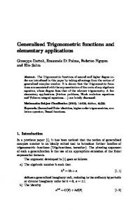
for n = 0, 1, 2. For x > 1, they are only slightly worse than the corresponding (and higher degree) lower bounds for ln(x) given by Daumas et al. We therefore use them for all x > 0. The current lack of range reduction means that our upper bounds are poor when x > 2 and similarly our lower bounds are poor when x < 1/2. This point is evident in Fig. 2, which plots ln(x) against the upper bound (2x3 − 9x2 + 18x − 11)/6 as x ranges from 0.1 to 3. Bounds of higher degree are actually worse as x increases. We are considering alternative logarithm bounds that may exhibit less extreme behaviour.

Fig. 2. An Upper Bound for the Logarithm Function

3.2

The Exponential Function

Daumas et al. [9] derive bounds for exp(x) from its Taylor expansion, but only for −1 ≤ x < 0. They use a complicated system of transformations, first covering the negative numbers in separate intervals of the form [k −1, k) for integer k < 0. For x > 0, they use the identity exp(−x) =

1 exp(x).

The rapid growth of the exponential function necessitates a degree of case analysis and range reduction, but we have managed to find simpler bounds valid over wide ranges. We use a crucial fact about the Taylor expansion [7, p. 83].

Proposition 2. If n is odd and x 6= 0 then exp(x) >

n X xi i=0

i!

.

If n is even then this inequality holds if x > 0, while the opposite inequality holds if x < 0. Obviously we have equality when x = 0.

Fig. 3. An Upper Bound for the Exponential Function

Our upper bounds for x ≤ 0 rely on this opposite inequality. The bound using n = 4 is already poor when x < −2, so they could benefit from range reduction, but they are valid for all x ≤ 0. Our upper bounds for x ≥ 0 rely on Prop. 2 with odd n. We define exp(−x) = 1/exp(x): dividing by a positive lower bound yields an upper bound. Obviously the exponential function is not bounded by any rational function for x > 0, and one might imagine that the exponential function overtakes its bound after a certain point. In fact, our upper bounds are never overtaken, but reach a discontinuity as the denominator goes to zero. With n = 3, the upper bound is 6/(6 − 6x + 3x2 − x3 ); its denominator is a cubic equation with one real root at x ≈ 1.60. The divergence of the upper bound function can be seen in Fig. 3, which plots exp(x) against the upper bound (dashed line) as x ranges from 0 to 1.5. We could get a much tighter fit by choosing n = 5, which diverges at x ≈ 2.18. Due to the limited range of these bounds, we also include a few versions with range reduction, via the identity exp(x) = exp(x/k)k , for k = 2, 3, 4. With k = 4 and n = 3, the denominator of the upper bound becomes a 12th degree polynomial.

Fig. 4. Lower Bounds for the Exponential Function

The treatment of lower bounds is simple, thanks to Prop. 2. The Taylor expansion of exp(x) for odd n is a valid lower bound over the entire real line. Figure 4 plots exp(x) against the lower bounds 1 + x (dashed line) and 1 + x + x2 /2 + x3 /6 (dotted line) as x ranges from −4 to 3. It is clear that the lower bounds are poor when x < −3. We can again use exp(x) = exp(x/k)k for range reduction, but only for odd k. We want to deduce exp(x/k)k ≤ exp(x/k)k = exp(x) from exp(x/k) ≤ exp(x/k), for which we need k to be odd because exp(x/k) could be negative. No single lower bound is uniformly best, so we use the Taylor expansion with n = 1, 3, 5 and 7. For n = 3 and n = 5, we also perform range reduction as described above with k = 3; the best of these bounds has degree 15 and is an excellent fit for −8 ≤ x ≤ 8. 3.3

Other Functions

For the functions sin(x), cos(x) and tan−1 (x), we use a selection of the bounds recommended by Daumas et al. [9]. They also suggest families of bounds that converge to π, but we cannot use families and have simply chosen two fractions based on the √ decimal expansion of π. We have improved the accuracy of their bounds for x while retaining their use of Newton’s method. We specify the absolute value function by a pair of clauses: ¬(0 ≤ x) ∨ |x| = x

0 ≤ x ∨ |x| = −x

Strengthening the second clause to 0 < x ∨ |x| = −x harms performance. The theorem prover uses these axioms to remove occurrences of the absolute value

function while introducing new literals of the form ¬(0 ≤ t) or 0 ≤ t. Presumably, it helps to make these literals complementary. 3.4

Axioms

The guiding principle behind our axiom system is to avoid all use of general properties of orderings, such as transitivity, antisymmetry and monotonicity of addition and multiplication. Necessary instances of these properties are built into other axioms, built into simplification or left to the decision procedure. To limit problem size and search space, we include only axioms that are relevant to the functions that appear in the problem. It is often obvious by inspection whether upper or lower bounds are required. At present the user has to convert the problem to clause form and to include the required sets of axioms, although these steps would be trivial to automate. A significant change from our previous paper [1] is that the less-than relation no longer exists. We have only one ordering relation, ≤. The equivalence X < Y ⇐⇒ ¬(Y ≤ X), formerly a pair of clauses, is now built into the parser. To illustrate our formalization of bounds, consider the fact 1 + x ≤ exp(x). We could combine it with transitivity for ≤ and < by asserting two axioms: ¬(Y ≤ 1 + X) ∨ Y ≤ exp(X) ¬(Y < 1 + X) ∨ Y < exp(X) However, writing each bound twice would be inconvenient. Instead we introduce a generalized less-than relation. Its first argument indicates which relation it designates. We express the following two equivalences using the obvious four axiom clauses: lgen(0, X, Y ) ⇐⇒ X ≤ Y lgen(1, X, Y ) ⇐⇒ X < Y Now, the lower bound axiom for ≤ and < can be expressed by a single clause: ¬(lgen(R, Y, 1 + X)) ∨ lgen(R, Y ≤ exp(X)). The theorem prover will then generate the two clauses shown above. We use weights and subterm coefficients to ensure that the exp literals are selected. The lower bound clauses combine with literals of the form ¬(t ≤ exp(u)) or ¬(t < exp(u)), respectively. These can substitute the lower bound in both conjectures and facts. – They reduce a conjecture of the form t ≤ exp(u) to t ≤ 1 + u, and similarly for 0; we also need axioms for Z < 0.

Table 1. Problems and Runtimes

problem −1 < x =⇒ 2|x|/(2 + x) ≤ 1 + |ln(1 + x)| |x| < 1 =⇒ |ln(1 + x)| ≤ − ln(1 − |x|) |x| < 1 =⇒ |x|/(1 + |x|) ≤ |ln(1 + x)| |x| < 1 =⇒ |ln(1 + x)| ≤ |x| (1 + |x|)/|1 + x| |x| < 1 =⇒ |x|/4 < |exp(x) − 1|

seconds 0.373 0.112 1.478 2.052 2.068

0 < |x| < 1 =⇒ |exp(x) − 1| < 7|x|/4 1.071 |exp(x) − 1| ≤ exp(|x|) − 1 1.760 |exp(x) − (1 + x)| ≤ |exp(|x|) − (1 + |x|)| 3.617 ˛ ˛ ˛ ˛ ˛exp(x) − (1 + x/2)2 ˛ ≤ ˛exp(|x|) − (1 + |x|/2)2 ˛ 27.802 0 ≤ x =⇒ 2x/(2 + x) ≤ ln(1 + x) 0.147 √ −1/3 ≤ x ≤ 0 =⇒ x/ 1 + x ≤ ln(1 + x) 0.241 2 3 2 1/3 ≤ x =⇒ ln((1 + x)/x) ≤ 2/3 + (12x + 12x + 1)/(12x + 18x + 6x) 0.216 √ 1/3 ≤ x =⇒ ln((1 + x)/x) ≤ 1/3 + 1/ x2 + x 0.528 0 ≤ x ≤ 1 =⇒ exp(x − x2 ) ≤ 1 + x 0.068 x ≤ 1/2 =⇒ exp(−x/(1 − x)) ≤ 1 − x 0.094 |x| < 1 =⇒ |sin(x)| ≤ 6/5|x| 0 < x < 100/201 =⇒ cos(πx) > 1 − 2x cos(x) − 1 + x2 /2 ≥ 0 0 < x ≤ π =⇒ cos(x) ≤ sin(x)/x 0 < y < x =⇒ (1/2) ln(x/y) > (x − y)/(x + y)

4

0.342 0.079 0.004 0.130 1.176

Results

Our previous paper presented a table of results for about 30 simple problems. As of this writing, we have 179 problems, which 68 percent are proved in under 60 seconds. For this paper, we present (Table 1) a small sample of the more

interesting and difficult problems. The runtimes were measured on a 2.66 GHz Mac Pro running Poly/ML. Limitations of our approach can be seen in the facts that cannot be proved. We cannot prove 2 > 2/(e(ln 2)2 ) or other problems in which functions are multiplied together. We can prove cos(πx) > 1 − 2x under the assumption 0 < x < 100/201 but unfortunately not under the assumption 0 < x < 1/2: our approximation to π is fixed and some precision is inevitably √ lost. Some problems involving square roots can be proved, but each square root E in the problems presented here has been manually replaced by a new variable y such that y ≥ 0 and y 2 = E. This transformation encodes square roots as algebraic constraints and can easily be automated. It is only useful if E is algebraic.

5

Conclusions

MetiTarski, which combines a resolution theorem prover with specialized simplification and a decision procedure, can prove numerous facts about the elementary functions automatically. By further refining our techniques, particularly for products of functions, we expect to prove increasingly difficult theorems. The approach is flexible, and should work with any well-behaved functions. Our objective is to perform proofs that could in principle be reconstructed or checked using other tools. Such reconstruction would be difficult however because QEPCAD performs lengthy computations using sophisticated algorithms. Our use of x/0 = 0 is well-known in interactive theorem proving. Although it is unconventional, it is logically consistent with traditional mathematics, which ascribes x/0 no value at all. Resolution is traditionally regarded first as a formal calculus and only second as an implementation. A resolution calculus is first developed, then proved to be complete, before an implementation is contemplated. Our choice of Metis could also be questioned. On this point, however, we have the support of SPASS+T implementer Uwe Waldmann: “switching to SPASS would make sense for you only if you plan to deal with huge problems” and we would spend a lot of time “getting memory (de)allocation right.”3 ML’s garbage collector certainly simplifies our task. Our results demonstrate that modifying an implementation can, at least, deliver proofs and insights. Our modifications are sympathetic to the overall architecture of resolution: we modify its notions of simplification and subsumption and its ordering. We ignore completeness because proving something is better than proving nothing. Nonetheless, we welcome suggestions for achieving completeness under particular circumstances. Acknowledgements. The research was funded by the epsrc grant EP/C013409/1, Beyond Linear Arithmetic: Automatic Proof Procedures for the Reals. Joe Hurd offered much help with his Metis prover. Christopher W. Brown and Ian Grant provided support for QEPCAD. John Harrison, David Lester, Cesar Muoz and Uwe Waldmann answered various queries. 3

E-mail dated 20 November 2007

References 1. B. Akbarpour and L. Paulson. Extending a resolution prover for inequalities on elementary functions. In Logic for Programming, Artificial Intelligence, and Reasoning, pages 47–61, 2007. 2. B. Akbarpour and L. C. Paulson. Towards automatic proofs of inequalities involving elementary functions. In B. Cook and R. Sebastiani, editors, PDPAR: Pragmatics of Decision Procedures in Automated Reasoning, pages 27–37, 2006. 3. F. Baader and T. Nipkow. Term Rewriting and All That. Cambridge University Press, 1998. 4. L. Bachmair and H. Ganzinger. Resolution theorem proving. In A. Robinson and A. Voronkov, editors, Handbook of Automated Reasoning, volume I, chapter 2, pages 19–99. Elsevier Science, 2001. 5. M. Beeson. Automatic generation of a proof of the irrationality of e. JSC, 32(4):333–349, 2001. 6. C. W. Brown. QEPCAD B: a program for computing with semi-algebraic sets using CADs. SIGSAM Bulletin, 37(4):97–108, 2003. 7. P. S. Bullen. A Dictionary of Inequalities. Longman, 1998. 8. E. Clarke and X. Zhao. Analytica: A theorem prover for Mathematica. Mathematica Journal, 3(1):56–71, 1993. 9. M. Daumas, C. Mu˜ noz, and D. Lester. Verified real number calculations: A library for integer arithmetic. On the Internet at http://hal.archives-ouvertes.fr/hal-00168402/fr/. 10. A. Dolzmann, T. Sturm, and V. Weispfenning. Real quantifier elimination in practice. Technical Report MIP-9720, Universit¨ at Passau, D-94030, Germany, 1997. 11. J. Harrison. Formalized mathematics. Technical Report 36, Turku Centre for Computer Science (TUCS), Lemmink¨ aisenkatu 14 A, FIN-20520 Turku, Finland, 1996. On the Internet at http://www.cl.cam.ac.uk/ jrh13/papers/form-math3.html. 12. H. Hong. QEPCAD — quantifier elimination by partial cylindrical algebraic decomposition. Sources and documentation are on the Internet at http://www.cs.usna.edu/ qepcad/B/QEPCAD.html. 13. L. H¨ ormander. The Analysis of Linear Partial Differential Operators II: Differential Operators with Constant Coefficient. Springer, 2006. First published in 1983; cited by Mclaughlin and Harrison [17]. 14. J. Hurd. Metis first order prover. http://gilith.com/software/metis/, 2007. 15. M. Ludwig and U. Waldmann. An extension of the Knuth-Bendix ordering with LPO-like properties. In N. Dershowitz and A. Voronkov, editors, Logic for Programming, Artificial Intelligence, and Reasoning, LPAR 2007, volume 4790 of Lecture Notes in Computer Science, pages 348–362. Springer, 2007. 16. W. McCune and L. Wos. Otter: The CADE-13 competition incarnations. Journal of Automated Reasoning, 18(2):211–220, 1997. 17. S. McLaughlin and J. Harrison. A proof-producing decision procedure for real arithmetic. In R. Nieuwenhuis, editor, Automated Deduction — CADE-20 International Conference, LNAI 3632, pages 295–314. Springer, 2005. 18. V. Prevosto and U. Waldmann. SPASS+T. In G. Sutcliffe, R. Schmidt, and S. Schulz, editors, FLoC’06 Workshop on Empirically Successful Computerized Reasoning, volume 192 of CEUR Workshop Proceedings, pages 18–33, 2006.