An Autonomic Failure-Detection Algorithm* K. Mills, S. Rose, S. Quirolgico NIST Mail Stop 892 Gaithersburg, Maryland 20899 1-301-975-3618 {kmills, scottr, steveq}@nist.gov
M. Britton Southern Methodist University 1265 Columbine Lane Salina, Kansas 67401 1-214-641-9914
[email protected]
ABSTRACT Designs for distributed systems must consider the possibility that failures will arise and must adopt specific failure detection strategies. We describe and analyze a self-regulating failuredetection algorithm that bounds resource usage and failuredetection latency, while automatically reassigning resources to improve failure-detection latency as system size decreases. We apply the algorithm to (1) Jini leasing, (2) service registration in the Service Location Protocol (SLP), and (3) SLP service polling.
C. Tan Montgomery Blair High School 403 Branch Drive Silver Spring, MD 20901 1-301-593-8132
[email protected]
TR = time of rising heartbeat
TF = time of falling heartbeat
HP = heartbeat period N = number of Monitorables
SR = size of rising heartbeat
Monitorable
Figure 2 defines the period of inconsistency when a monitorable fails between heartbeats. Should a monitorable fail immediately after receiving a falling heartbeat from a monitor, then the maximum failure-detection latency (LMAX) is defined by the heartbeat period, i.e., LMAX = HP. Assuming a monitorable is equally likely to fail at any time, the average failure-detection latency (LAVG) is half the heartbeat period, LAVG = HP/2. *This work is a contribution of the U.S. Government, not subject to copyright. In addition, the work identifies certain commercial products and standards to describe our study adequately. The National Institute of Standards and Technology neither recommends nor endorses these products or standards as best available for the purpose.
TR
Falling Heartbeat
TF
Rising Heartbeat
TR + HP
Falling Heartbeat
. . .
TF + HP
Rising Heartbeat TF + i * HP
TR + i * HP
Falling Heartbeat
Bandwidth Usage (B) B = N (SR + SF ) / HP
Figure. 1. Fundamental outlines of a two-way, heartbeatbased, failure-detection technique. Monitorable
2. AUTONOMIC FAILURE-DETECTION Figure 1 illustrates a two-way heartbeat failure-detection technique, where N monitorables each issue a rising heartbeat (every HP seconds) to one monitor, which replies with a falling heartbeat. Assuming rising and falling heartbeat messages of known size (SR and SF, respectively), the system consumes network bandwidth B = N (SR+SF)/HP. The monitor must process N/HP heartbeat messages per second. The monitorable must process 1/HP heartbeat messages per second.
Monitor Rising Heartbeat
1. INTRODUCTION Recent research on failure detection and recovery in distributed systems reports non-functional periods comprising two distinct phases: periods when a system is unaware of a failure (failuredetection latency) and periods when a system attempts to recover from a failure (failure-recovery latency)[1]. Depending on system architecture and assumptions about failure characteristics of components, the study found failure-detection latencies covered from 55% to 80% of non-functional periods. The study also revealed failure detection can consume substantial overhead. These findings suggest distributed systems could benefit from failure detection algorithms that exhibit definite bounds on latency and overhead. We define and analyze such an algorithm, and then apply it to Jini leasing and to service registration and polling in SLP.
SF = size of falling heartbeat
Monitor Rising Heartbeat
TF
Falling Heartbeat
TR
FAILURE LATENCY (L)
LAVG = HP / 2
DETECTION
TR + HP
LMAX = HP
Figure 2. Defining failure-detection latency for heartbeat-based failure-detection techniques. For monitor failure, where detection occurs when the monitor does not respond with a falling heartbeat, the situation differs slightly. A monitorable may wait for some timeout period (TO) before concluding the monitor has failed; thus, the maximum detection latency for monitor failure is HP + TO, and the average detection latency is HP/2 +TO. We define an autonomic algorithm to limit bandwidth usage to an allocated capacity (BA) and to limit average failure-detection
200
NMAX Number of Monitorables (N)
latency (to LWORST), while reducing average failure-detection latency (LAVG < LWORST) to some lower bound (LBEST) when the number of monitorables (N) falls below system capacity (NMAX). We modify the two-way heartbeat technique so that the monitor includes a heartbeat period (HP) in each falling heartbeat. The monitorable uses HP to determine when to issue the next rising heartbeat. The monitor may vary HP with each falling heartbeat to maintain an operating range defined by three policy goals: the average failure-detection latency in the worst (LWORST) and best (LBEST) cases and the allocated bandwidth (BA).
150
N
N
100
50
0
Assuming N monitorables, the monitor varies the heartbeat period (HMIN < HP < HMAX) using the algorithm in Figure 3.The maximum heartbeat period (HMAX) is set to twice the worst-case average failure-detection latency (HMAX = 2 LWORST). Given HMAX and the monitor’s capacity [C = BA/(SR + SF)], a monitor can watch at most NMAX = HMAX C monitorables. Assuming a monitor watches at least one monitorable, a natural choice for HMIN would be 1/C; however, this heart rate might place too great a load on individual monitorables. Instead, we choose a best-case goal (LBEST) for average failure-detection latency and set HMIN = 2 LBEST. HMIN establishes a lower bound on failure-detection latency. Below, we report analytical results as time-series plots (time increases from 0 to 400) with N first increasing to 200, and then decreasing back to 0. In all plots (Figure 4) we assume the same heartbeat sizes (SR = 128 bytes and SF = 64 bytes) and policy goals (LWORST = 30 s, LBEST = 7.5 s, and BA = 576 bytes/s). The top plot shows our algorithm limits monitor workload to NMAX, while the second plot illustrates our algorithm adjusting HP between HMIN and HMAX as N varies. The third plot shows how average bandwidth increases and decreases but never exceeds allocated bandwidth (BA). The bottom plot illustrates how our algorithm improves average failure-detection latency (L) as N decreases (ticks 200 to 400), while average failure-detection latency never exceeds the worst (LWORST) and best (LBEST) cases.
3. SAMPLE APPLICATIONS We apply our algorithm to selected functions in two servicediscovery protocols: Jini [2] and the Service Location Protocol (SLP) [3]. Jini enables clients and services to rendezvous through a third party, known as a lookup service. Each Jini service registers a description of itself with each discovered lookup service, and requests a lease duration (LR), which may be accepted at time TG for a granted lease period LG < LR. LR may be “any”, which allows a lookup service to assign any value for LG. To extend registration beyond LG, services must renew the lease prior to an expiration time TE = TG + LG; otherwise, registration is
100
200
300
400
Time
Heartbeat Period (HP ) in Seconds
75
HMAX 50
HP
HP
25
HMIN
HMIN
0 0
100
200
300
400
Time
Bandwidth Consumption (B) in B/s
Figure 3. Autonomic algorithm to vary heartbeat period.
0
600
BA
500 400
B
B
300 200 100 0 0
100
200
300
400
Time
Failure-Detection Latency (L) in Seconds
if new monitorable then N++; HP = N / C; if HP > HMAX then N--; raise capacity exception; elseif HP < HMIN then HP = HMIN ; endif endif
40
LWORST
32
24
L 16
8
LBEST
0 0
100
200
300
400
Time
Figure 4. Time-series plots from an analytical model of the proposed autonomic failure-detection algorithm. revoked. This cycle continues until a service cancels or fails to renew a lease. Lookup services assign LG within a configured range, LMIN < LG < LMAX. While a granted lease may not be revoked prior to TE, lookup services may deny any lease request.
SLP Service Registration. SLP enables clients, called user agents (UAs), and services, called service agents (SAs), to rendezvous through a third party, known as a directory agent (DA). A SLP SA registers a description of itself with each discovered DA. A UA may query any discovered DAs to find services of interest and to obtain attributes that describe services. A SA requests registration for a time-to-live (TTLR), which may be accepted by a DA at time TG. To extend registration beyond TTLR, the registering SA must renew the registration prior to an expiration time TE = TG + TTLR; otherwise, the DA revokes the registration. This cycle continues until the SA cancels or fails to refresh a registration. While an accepted registration may not be revoked prior to TE, a DA may deny any registration request. A DA will always deny a registration request when TTLR is too small, as determined by comparing the TTLR against a minimumrefresh interval (RFMIN) included within advertisements multicast by the DA at a periodic rate (DABEAT). We apply our algorithm to provide SLP service registration with rapid feedback, eliminating the need for RFMIN. We add a field (TTLG) to the SrvAck message, used by DAs to acknowledge service-registration (SrvReg) messages from SAs. Then, a DA can ignore TTLR and instead compute a granted timeto-live (TTLG), which can vary dynamically within a bounded range (TTLMIN < TTLG < TTLMAX) while limiting resource consumption associated with refreshing service registrations. The
Number of Registered Services (N)
150 100 50 0 0
100
200
300
400
300
400
300
400
Lease Grant Period (LG) in seconds
75 50 25 0 0
100
200 Time
Bandwidth Used (B) in Bytes/Second
To verify our analysis, we implemented our algorithm in a Jini simulation and compared simulation results against analytical predictions, given a selected set of policy goals and known sizes for Jini messages. We subsequently implemented our algorithm in a publicly available implementation of the Jini lookup service. We modified the lookup service code to accept our policy goals and to measure and report average bandwidth usage (B), the number of registered services (N), and the value for LG. We deployed our modified Jini lookup service in a test bed built to control and monitor thousands of Jini services. We coded a measurement client to detect service arrivals and departures, computing average failure-detection latency (L). We measured behavior of a live Jini system using the same policy goals selected for analysis and simulation. We report our results in Figure 5 as four time-series plots, where we used the same protocol parameters (SR = 350 bytes and SF = 350 bytes) and policy goals (BA = 2100 bytes/second, LBEST = 7.5 seconds and LWORST = 1200 seconds, and so NMAX = 7200) for the analysis, the simulation (1000 repetitions per data point), and the live system (20-30 repetitions per data point).
200
Time
Simulation
2500 2000 1500
Analysis
1000
Measurement
500 0 0
100
200 Time
Failure-Detection Latency (L) in Seconds
We apply our algorithm to enable Jini lookup services to vary LG within a bounded range (LMIN < LG < LMAX) while limiting resource consumption associated with lease renewal. The mapping is straightforward. Assuming three policy goals, bandwidth allocated (BA) and worst (LWORST) and best (LBEST) failure-detection latencies, we compute LMIN = HMIN = 2 LBEST and LMAX = HMAX = 2 LWORST. Knowing the size of the rising (lease request) and falling (lease grant) heartbeats (SR and SF, respectively), leasing capacity (C) is computed as before. Knowing the number of registered services (N), a Jini lookup service uses the algorithm in Figure 3 to compute HP and then uses that value as the granted lease period (LG = HP). If the new lease would exceed system capacity, then the lookup service issues a LEASE_DENIED exception.
Measurement
40 30
Simulation
20
Analysis
10 0 0
100
200
300
400
Time Figure 5. Time-series plots showing application of autonomic failure-detection to Jini leasing procedures
mapping is straightforward. Assuming our three policy goals, bandwidth allocated (BA) and worst (LWORST) and best (LBEST) failure-detection latencies, we compute TTLMIN = HMIN = 2 LBEST and TTLMAX = HMAX = 2 LWORST. Knowing the size of the rising (SrvReg) and falling (SrvAck) heartbeat messages (SR and SF, respectively), registration capacity (C) is computed as before.
SLP UA Polling. SLP UAs must poll DAs periodically to learn about service arrivals and departures or about changes in attribute values of service descriptions. SLP includes no mechanisms through which DAs can control the polling rate of UAs. We can modify DA procedures to determine which UAs are polling a DA, and then we can apply our algorithm to assign polling intervals to those UAs. First, we explain the modified DA procedures. When a UA queries a DA, either using a service-request (SrvRqst) or attribute-request (AttrRqst) message, we modify the DA procedures to lookup the UA in a local DA cache. If the UA is not found, then the DA creates a new cache entry for the UA; otherwise, the DA uses the existing cache entry. The DA grants the cache entry a polling interval (PG), which can vary dynamically within a bounded range (PMIN < PG < PMAX) while limiting resource consumption associated with UA polling. We modify the format of the appropriate reply message, either the service reply (SrvRply) or the attribute reply (AttrRply), to include a field to hold PG for return to the UA. If the UA fails to issue another query to the DA by the time PG expires, then the DA purges the associated entry from the local cache of UAs. Upon receiving PG in the reply message, the UA schedules its next poll (if any) of the DA to occur slightly before PG expires. The DA can use our algorithm to determine a suitable value for PG. The mapping is straightforward. Assuming our three policy goals, bandwidth allocated (BA) and worst (LWORST) and best (LBEST) failure-detection latencies, we compute PMIN = HMIN = 2 LBEST and PMAX = HMAX = 2 LWORST. Estimating an average size for the rising (SrvRqst or AttrRqst) and falling (SrvRply or AttrRply)
Number of Registered Services (N)
200 150 100 50 0 0
100
200
300
400
300
400
300
400
300
400
Time-To-Live Granted (TTLG) in Seconds
Time
Bandwidth Used (B) in Bytes/Second
To verify our analysis, we implemented our algorithm in a SLP simulation and compared simulation results against analytical predictions. We report our results in Figure 6 as four time-series plots, where we used the same protocol parameters (SR = 76 bytes and SF = 56 bytes) and policy goals (BA = 396 bytes/s, LBEST = 7.5 seconds and LWORST = 500 seconds) for the analysis and the simulation. Setting LWORST = 500 seconds and BA = 396 bytes/s provides a maximum system capacity of NMAX = 3000 registered services. In the main, Figure 6 shows a close correspondence between analytical predictions and simulation results; however, the bandwidth-usage simulation plot (as well as the bandwidthusage simulation plot for Jini leasing procedures - recall Figure 5) illustrates a hysteresis within the control loop of our proposed algorithm. During periods of increasing system size, the algorithm typically assigns a heartbeat period that immediately becomes too small for the now increased system size, and will only be able to reduce the heartbeat period one monitorable at a time, as each previously assigned heartbeat expires. This lag causes the algorithm to slightly overshoot the allocated bandwidth. The larger the heartbeat message size the greater the overshoot. For example, the Jini plot (700 bytes per heartbeat) overshoots allocated bandwidth more than the SLP plot (132 bytes per heartbeat). However, the downward slope in the bandwidth-usage simulation plots (as system size increases from 50 to 200) suggests that the algorithm will stabilize bandwidth usage at the allocated bandwidth once the system size stabilizes.
heartbeat messages (SR and SF, respectively), registration capacity (C) is computed as before. Knowing the number of polling clients
75
50
25
0 0
100
200 Time
Simulation
500 400 300
Analysis
200 100 0 0
100
200 Time
Failure-Detection Latency (L) in Seconds
Knowing the number of registered services (N), a DA can use the algorithm in Figure 3 to compute HP and then use that value as the granted time-to-live (TTLG = HP). If a new registration would exceed system capacity, then the DA issues the SrvAck with a status code of DA_BUSY_NOW.
40 30 20 10 0 0
100
200 Time
Figure 6. Time-series plots showing application of autonomic failure-detection to SLP serviceregistration refresh procedures (N), a DA can use the algorithm in Figure 3 to compute HP and
Figure 7 shows a close correspondence between analytical predictions and simulation results, and also again illustrates the hysteresis associated with the bandwidth-allocation control loop. Here, the overshoot is worse than for SLP service registration because the SLP polling heartbeat message sizes are greater (205 bytes on average compared with 132 bytes). The bandwidth-usage overshoot is lower than for Jini leasing, however, because the SLP polling heartbeat messages are smaller (205 bytes on average compared with 350 bytes). Further, the overshoot for SLP polling is somewhat exaggerated because the initial four-message exchange prior to the polling heartbeats is included in the bandwidth-usage during periods of increasing system size. This can also be seen in the results from our modified analytical model, which overshoots the allocated bandwidth (615 bytes/s). This effect diminishes as the granted polling interval (PG) increases, as can be seen in the downward slope in both the analytical predictions and simulation results.
4. REFERENCES [1] C. Dabrowski, K. Mills, and A. Rukhin A. Performance of Service-Discovery Architectures in Response to Node Failures, Proceedings of the 2003 International Conference on Software Engineering Research and Practice (SERP'03), CSREA Press, June 2003, pp. 95-101.
[2] K. Arnold et al, The Jini Specification, V1.0 AddisonWesley 1999. Latest version is 1.1 available from Sun.
Number of Polling Clients (N)
100 50 0 0
100
200
300
400
300
400
Time Polling Interval Granted (PG) in Seconds
We report our results in Figure 7 as four time-series plots, where we used the same protocol parameters (average SR = 77 bytes and average SF = 128 bytes) and policy goals (BA = 615 bytes/s, LBEST = 7.5 seconds and LWORST = 500 seconds) for the analysis and the simulation (1000 repetitions per data point). Setting LWORST = 500 seconds and BA = 615 bytes/s provided a maximum system capacity of NMAX = 3000 registered services. For the simulation, we sampled individual message sizes from a distribution for each AttrRqst and AttrRply. The distribution parameters for an AttrRqst were: 4 bytes minimum, 256 bytes maximum, 77 bytes average, and 138 bytes variance. The distribution parameters for an AttrRqst were: 64 bytes minimum, 224 bytes maximum, 128 bytes average, and 25 bytes variance.
150
75
50
25
0 0
100
200 Time
Bandwidth Used (B) in Bytes/Second
To verify our analysis, we implemented our algorithm in a SLP simulation and compared simulation results against analytical predictions, given a selected set of policy goals and estimated sizes for SLP messages. We devised a specific polling algorithm. Upon discovering a DA, a UA first issues one SrvRqst message (receiving a SrvRply from the DA) and then an AttrRqst message (receiving a AttrRply from the DA). The DA grants a PG only for each AttrRply message, and the UA polls only with AttrRqst messages. In other words, on initial discovery a UA and DA exchange four messages (SrvRqst-SrvRply-AttrRqst-AttrRply), and then the UA and DA periodically exchange two messages (AttrRqst-AttrRply). We modified our analytical model to account for these polling procedures.
200
800
Failure-Detection Latency (L) in Seconds
then use that value as the assigned polling interval (PG = HP). If a new polling UA would exceed system capacity, then the DA issues the SrvRply or AttrRply with a status code of DA_BUSY_NOW.
40
Simulation
600 Analysis
400 200 0 0
100
200
300
400
Time
30 20 10 0 0
100
200
300
400
Time
Figure 7. Time-series plots showing application of autonomic failure-detection to SLP UA polling
[3] Service Location Protocol Version 2, Internet Engineering Task Force (IETF), RFC 2608, June 1999.