An Autonomic Tool for Building Self-Organizing Grid ... - CiteSeerX

An Autonomic Tool for Building Self-Organizing Grid-enabled Applications Gianluigi Folino and Giandomenico Spezzano ∗ Institute of High-Performance Computing and Networking (ICAR) National Research Council (CNR), Italy Via Pietro Bucci 41C, I-87036 Rende (CS), Italy

Abstract In this paper we present CAMELotGrid, a tool to manage Grid computations of Cellular Automata that support the efficient simulation of complex systems modeled by a very large number of simple elements (cells) with local interaction only. The study of these systems has generated great interest over the years because of their ability to generate a rich spectrum of very complex patterns of behavior out of sets of relatively simple underlying rules. Moreover, they appear to capture many essential features of complex self-organizing cooperative behavior observed in real systems. The middleware architecture of CAMELotGrid is designed according to an autonomic approach on top of the existing Grid middleware and supports dynamic performance adaptation of the cellular application without any user intervention. The user must only specify, by global criteria, the high level policies and submit the application for execution over the Grid. Key words: Grid computing, autonomic computing, cellular automata

1

Introduction

The emergence of Computational Grids [12] as the next generation distributed computing platform has enabled a new generation of applications based on seamless access, aggregation and interaction. For example, it is possible to conceive a new generation of scientific and engineering simulations of complex physical phenomena that combine computations, experiments, observations, and real-time data and can provide important insights into complex systems ∗ Corresponding author. Email address: [email protected] (Giandomenico Spezzano).

Preprint submitted to Elsevier Science

22 November 2006

such as road traffic, image processing, landslide simulation and science of materials. Many of these phenomena have been successful modeled and simulated by cellular automata (CA)[24]. CA are mathematical models for complex natural systems containing large numbers of simple identical components with local interactions. They consist of a lattice of sites, each with a finite set of possible values. The value of the sites evolve synchronously in discrete time steps according to identical rules. The value of a particular site is determined by the previous values of a neighborhood of sites around it. CA are discrete dynamical systems with simple construction but complex self-organizing behavior. Current CA packages are either specialized single node programs or they are programming environments for building parallel applications. Today, with the current trend for larger scale CA problem solutions, we need Grid-enabled implementations of CA. Computational Grids provide the software and networking infrastructure to harness a heterogeneous environment that includes geographically distributed computer domains, to form a massive computing environment through which large scale problems can be solved. To achieve this goal, Grids need to support various tools and technologies that can guarantee security, uniform access, resource management, scheduling, application composition, computational economy and accounting [3]. Realizing software systems on the Grid requires not only the knowledge of standards such as OGSA (Open Grid Services Architecture) and tools like Globus [11], but also sophisticated paradigms that effectively hide the complexity of creating and deploying truly parallel Grid applications in presence of dynamicity, adaptivity and fault tolerance. High level problem solving environments (PSEs) provide a general, uniform framework allowing researchers to concentrate on their specific system of interest without being involved in the lower level parallelization tasks. However, building PSEs in a computational grid infrastructure [26,19] is a challenging task because the concurrent program, which represents the runtime of the application, must dynamically adapt to changing resource availability in the grid environment. Supporting dynamically configurable programs requires a programming paradigm and management techniques that deal with complexity, heterogeneity and uncertainty. This has led researchers to consider alternative programming paradigms based on the strategies used by biological systems that exhibit a self-organizing behavior and that have been recognized suitable for managing distributed resources. A significant bio-inspired paradigm has been defined by IBM in its ”Autonomic Computing” program [16]. An autonomic computing system is a system 2

which has the capabilities of being self-defining, self-healing, self-configuring, self optimizing, etc. and is able to manage itself without involving the user, in the same way the autonomic nervous system regulates the body systems without conscious input from the individual. The user must only specify, by global criteria, the high level policies (runtime partitioning strategies, etc.) and submit the application for execution over the Grid. In this paper, we present CAMELotGrid, the Grid-enabled version of the Camelot (Cellular Automata environMent for systEms ModelLing open technology) PSE developed in the Esprit project COLOMBO [18,8]. CAMELotGrid is a new middleware designed on top of the existing Grid middleware, which uses autonomic Grid functionality to intelligently manage problem partitioning, problem piece deployment, runtime management, dynamic level of parallelism, dynamic load balancing, and, in future, even fault tolerance and recovery. The remainder of this paper is organized as follows. Section 2 briefly presents an overview of Camelot. Section 3 and 4 describe how to specify autonomic requirements of a cellular application and the middleware architecture of CamelotGrid. Section 5 illustrates the performance model for predicting application execution time and in section 6 we evaluate the application performance using a landslide cellular model. Section 7 concludes with a summary.

2

Camelot overview

Camelot is a high performance simulation environment based on the CA formalism [25]. In our approach, a cellular algorithm is composed of all the transition functions of the cells that compose the lattice. Each transition function generally uses the same local rule, but it is possible to define some cells with different transition functions (heterogeneous cellular automata). Unlike early cellular approaches, in which cell state is defined as a single bit or a set of bits, we define the state of a cell as a set of typed sub-states. This allows extending the range of applications that can be programmed by cellular algorithms. Furthermore, we introduce a logic neighborhood that may represent a wide range of different neighborhoods inside the same radius and that may also be time-dependent. We have also implemented some mechanisms to observe and control the evolution of the automaton. The CAMELot simulation environment consists of: • a graphic user interface (GUI) for editing, compiling, configuring, executing, visualizing and steering the computation. The GUI allows, by menu pops, to define the size of the CA, the number of the processors on which the automaton must be executed, and to choose the colors to be assigned to the 3

cell sub-states to support the graphical visualization of their values; • a software library to integrate raster GIS images into the CA. The raster information can consist of different variables such as altimetry, soil, temperature, vegetation, etc. In CAMELot these variables are associated with the sub-states where the transition function provides a dynamic alteration of the information. For instance, the temperature values can be changed by a simple model that updates the temperature with regard to the hour of the day; • a load balancing algorithm similar to the scatter decomposition technique to evenly distribute the computation among processors of the parallel machine; • a language, called CARPET [7], which can be used to define cellular algorithms and to perform steering commands when complex space and time events are detected. CARPET is a language to program cellular algorithms and contains constructs to extend the range of interaction among the cells, introducing the concept of region, and to define algorithms to perform computational steering. It is a high-level language based on C with additional constructs to describe the rule of the state transition function of a single cell of a cellular automaton and to steer the application. A CARPET program is composed of a declaration part that appears only once in the program and must precede any statement, a body program that implements the transition function, and a steering part that contains a set of commands to extract and analyze system information and to perform steering. Figure 1 shows an example of application of these constructs. Two 3D regions are defined in a three-dimensional cellular automaton. The event expression checks whether the maximum and the minimum of the rainfall sub-state in a region(zone1) are equal. In case they are, the computation is stopped. If the sum of the rainfall values in another region(zone2) is greater than a threshold, then the value of the alpha parameter is changed. In any case, the computation is stopped after 10000 generations.

3

CAMELotGrid: an autonomic PSE

CAMELotGrid [8,6] is a PSE that provides a complete integrated computing environment for CA programming, permits to specify the global criteria defining the autonomic requirements of the application and to support the execution of cellular applications over the Grid. It extends the original CAMELot architecture for incorporating the features of self-configuring, self-optimizing, self-healing, etc., of an autonomic system, in order to realize a Grid-enabled middleware architecture where the runtime autonomic management of the application is done without any user intervention. 4

cadef { .... state (float rainfall, infiltration); parameter (alpha 2.0, ....); ..... region (zone1(10:20, 1:30, 5:50), zone2(1:4, 3:10, 1:50)); } ..... steering { if (step > 10000) cpt abort(); if (region max(zone1, rainfall) == region min(zone1,rainfall) cpt abort(); else if (region sum(zone2, rainfall) > Threshold) cpt set param(alpha, 3.5); ..... }

Fig. 1. An example of use of steering commands in CARPET.

In CAMELotGrid a spatio-temporal problem can be modeled by a 2D or 3D array of cells where each cell represents a portion of a landscape. By CARPET a user can describe, using the declaration, body and steering part, the transition function that represents the cellular program of the complex phenomenon that he/she intends to model. To support the development of autonomic applications we have extended CARPET with a new part, called autonomic. In the autonomic part, a user can define a set of rules to specify high level policies that capture different aspects of autonomic behavior. The rules defined in the autonomic part are used to manage the runtime behavior of the system. Rules incorporate high-level guidance and practical human knowledge in the form of event-condition-action (ECA) control structure. ECA rules are usually written in the following form: on event (if conditions) then actions (else actions) where event represents the event which should ignite the evolution of the baselevel system, conditions, and actions, respectively, represent the conditions the run-time support must validate when the event occurs and the actions the run-time support must carry out for adapting the system against the occurred event. An event can be any change in resources availability over time while the application is executing. For example, new processing nodes may become available or required for higher priority tasks; links may become overloaded, influencing the application performances. In all these cases, actions should be defined to adapt the run-time behavior of the algorithm to the current computation workload. In this section, we demonstrate how CARPET can be used to enable autonomic self-managing behavior in cellular applications. We focus on two aspects of self-management: self-configuration and self-optimization of the deployed system. Cellular autonomic applications can dynamically reconfigure themselves to 5

tackle the variation of availability and performance of grid platforms over time. Application adaptation is automatically triggered by changes of environmental status. Furthermore, applications should continually seek opportunities to improve their own performance and efficiency. Figure 2 shows an example of the autonomic part of CARPET. In the example, for every event occurs in the system the runtime system of CARPET is notified in order to decide whether an ECA rule will be triggered by that or not. If a rule is triggered a redistribution or a reconfiguration of the cellular automata will be executed. The program supposes that the user imposes to execute a cellular program with an efficiency value equal to 0.7 using a virtual machine (VM) with k nodes selected among the current resources (i.e. processors available) of the Grid. When some nodes become overloaded the efficiency can decrease so to keep the efficiency above the predefined threshold, if the number of processors belonging to the VM does not change, a redistribution of the automata must be performed. The redistribution involves a dynamic reallocation of some portions of the automata, without to stop the running system, from the overloaded nodes to the more unloaded nodes. The efficiency value (computed using the performance model described in section 5) is evaluated at run-time and automatically updated. In the case that at the most three nodes fail or the execution time, measured by a sensor at run-time, becomes greater than a predefined threshold the automata must be reconfigured. Reconfiguration is a more complex action that is performed for fault tolerance or self-optimization purposes. During the reconfiguration cycle a checkpoint of the automata is built, the internal process state is saved, the execution is frozen, new optimized executables are built and the application is re-launched.

....... steering { ...... } autonomic { on (efficiency < 0.7) if ((cardinality (VM )== k ) then redistribute(); on (failure (VM ) k responseTime > 2)) if (cardinality (VM ) >= (k -3 )) then reconfigure() else stop ; }

Fig. 2. An example of use of autonomic section in CARPET.

6

4

CAMELotGrid Architecture

In CAMELot, the run-time support was implemented as a SPMD (Single Program, Multiple Data) program. The latest implementation is based on the C language plus the standard MPI library and can be executed on different parallel machines and clusters of workstations. The concurrent program that implements the architecture of the system is composed by a set of macrocell processes, an execution engine and a GUI process. Each macrocell process, that operates on a strip of cells of the CA, runs on a single processing element of the parallel machine and updates the state of cells belonging to its partition.

The synchronization of the automaton and the execution of the commands, provided by a user through the GUI interface or described in the steering section, are carried out by the execution engine. The execution engine partitions the 2 or 3D cellular space according to the indications of the user and assigns the portion of the cells that must be processed to each macrocell process.

We extended the CAMELot architecture to support the development of autonomic cellular applications on the Grid. CAMELotGrid is the new middleware architecture that is implemented on existing Grid middleware and runtime services. An overview of the CAMELotGrid middleware architecture is shown in the figure 3. The Grid middleware layer takes advantage of the services offered by the Globus Toolkit [11], by the MPICH-G2[13] library, a grid-enabled implementation of the MPI v1.1 standard, and by the Network Weather Service (NWS) [21,22], a monitoring system to forecast short term network performance. In particular, NWS provides accurate forecasts of dynamically changing performance characteristics from a distributed set of metacomputing resources. MPICH-G2 uses services (e.g., job startup, security) provided by Globus to coordinate and manage work on multiple computer systems, potentially of different architectures.

The main components of the CAMELotGrid infrastructure architecture include the CAMELotGrid Manager (CGM), the Computational Resource Manager (CRM), the Application Performance Model (APM), and the Execution Engine (EE).

In what follows, we will describe how an application submitted by the user will use the CAMELotGrid infrastructure services to exploit the heterogeneous Grid resources and to achieve autonomic runtime management. 7

Fig. 3. The CAMELotGrid middleware architecture.

4.1 Deployment Strategy

The main administrative component in the CAMELOTGrid architecture is CGM, which is the autonomic application manager that sets up and configures/reconfigures the application execution environment, manages and controls all the autonomic requirements (e.g., self-configuring, self-optimizing, etc.) through the ECA rules defined in the autonomic section of CARPET. CGM is started by the GUI interface when the user wants to execute a new application. Before to start the execution of the distributed application, CGM must determine a valid configuration and to load the macrocell processes onto the chosen remote hosts. CGM uses the performance model defined in the APM module and described in the section 5, to choose the most appropriate pool of resources to schedule the components of the application. The performance model allows to predict the lowest estimated application execution time on a given set of resources with a given topology. The resource information, including the number of current available computation resources and their usage, necessary to feed the performance model are provided by the CRM module to CGM. Using these information CGM, assisted by APM, identifies a subset of the available resources to constitute the VM on which the application will be executed, calculates a mapping of 8

data and/or tasks to those resources and provides the best schedule for the macrocell processes. Finally, CGM starts the EE module. The EE module generates the processes required to simulate the model on each the defined subspaces and deploys the application. EE communicates to CGM and CRM information about the status of the computation of the automaton and its eventual termination. Furthermore, on request of CGM, EE can save or load a configuration of the automaton, abort and restart the computation with a new mapping and schedule (see next section).

4.2 Autonomic Runtime Management Strategy During the execution of a cellular application, CAMELotGrid is capable of dynamically managing, adapting and optimizing its behaviour to dynamic changes in the Grid environment (e.g. workload) and scale well (e.g. in terms of the size of applications). CAMELotGrid can be dynamically reconfigured by the CGM module. CGM uses an adaptive scheduling algorithm based on the same policy used by GRADS [2]. CGM receives notifies by CRM on any change of the network resources. CRM is an active module able to analyze the information coming from the Grid infrastructure. For example, CRM can determine if the network is congested or if new nodes are available in the Grid environment. CRM supports information collection by the two most widely used Grid resource information systems, the Metacomputing Directory Service (MDS) and NWS. MDS collects and publishes system configuration, capability, and status information such as operating system, processor type and speed, number of available CPUs, and the software installed. The information that can typically be retrieved from a NWS server include the fraction of CPU available to a newly started process, the amount of memory that is currently unused, and the bandwidth in which data can be sent/received to/from a remote host. Each dynamic variation notified by CRM triggers an event that control whether the application is delivering an acceptable level of performance (e.g. a level of efficiency). The evaluation of acceptable levels of performance is the shared responsibility of the APM module and the CGM module. To this aim, CGM uses the autonomic section of CARPET which contains rules that define actions to be executed when specified conditions are satisfied. During the execution, if CGM determines that the application is not making reasonable progress with respect to the defined policies (or alternatively, if the 9

system becomes aware of more suitable execution resources), a rescheduling action can be invoked. Examples of rescheduling actions are replacing particular resources, redistributing the application workload/task on the current resources, and adding or removing resources, or doing nothing (continuing execution with the current VM). Basing on the knowledge of the current execution, CGM determines the best course of actions in order to improve progress. Mainly, we can answer to changes in the environment with two kinds of actions: redistribution and reconfiguration. The first action requires a more simple policy: consider the case in that the load is unbalanced, as, for instance, new jobs are started on any processors of the VM. Then, CGM can redistribute the load, moving portion of the automata from more loaded machines to less loaded ones , using the information coming from CRM. A similar policy has been adopted in the Dynamite system [14]. The latter action is due to a failure in any resources belonging to the virtual machine or it can be a consequence of new available processors potentially can increase the efficiency of the VM. To reconfigure the application, CGM must checkpoint the run-time support (sending a message to EE to save the current configuration), make changes to the plan execution that may imply addition, removal, migration or replacement of components. Finally, after to have load the checkpoint information, the program continues the execution. Clearly, in order to make this execution scenario work, we must have a reasonable performance model and mapping strategies for each cellular application. In the next section, we present the performance model used in CAMELotGrid.

5

Performance Model

In this section, we describe the performance model used by APM to evaluate the performance application. The performance model is an analytic metric for predicting application execution times on a given set of resources with a defined communication topology. On a sequential machine we can model the execution time for one time-step of the cellular automaton, where a, b, c are the CA dimensions, as:

Ts = tas + abc

10

tf + tup Cl

where tf is the average computation time required to perform a transition function at a single grid point, tas is the average time required to perform some simple initialization operations, tup is the time necessary to update the cellular space with new values and Cl is the percentage of cpu load available t +t to the application. So, defining t0f = f Cl up we have: Ts = tas + abct0f

(1)

Now, consider a pool of resources with different computing power and different t +t cpu load (Grid computing environment). Define t0f (i) = f (i)Cl(i)up(i) where the symbols are the same used before, concerning the ith processor as explained in table 1. Table 1 Main symbols used in the model. a

Width of the automata

b

Height of the automata

c

Depth of the automata

d

substate dimension in bytes

P

number of processors

tf (i)

avg. exec. time of the transition function on the ith proc.

Cl (i)

perc. of cpu load available to the application on the ith proc.

ts (i, i + 1)

start-up time for comm. from the ith proc. to i + 1th proc.

tb (i, i + 1)

time to send a byte for comm. from the ith proc. to i + 1th proc.

tas (i)

additive sequential time on the ith proc.

tap (i)

additive parallel time on the ith proc.

1 t0f (i)

Define fi =

as an index of computing frequency of the processor ith . At

this point, we can compute the total frequency as f =

Pp

i=1

fi and αi =

fi . f

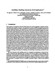
So we can balance the computing load, decomposing the cellular automata along the longer direction (see figure 4 that uses a decomposition along the x axis) and assigning to each node a sub-grid of dimension aαi bc. The computational load for processor will be abc . f Each processor has allocated a task performing the same computation on each point and at each time step. Each sub-grid is bordered in order to allow a local selection of the neighbors. The main operations of the distributed algorithm for the run-time execution of the CA are summarized in figure 5. The total execution time of the distributed CA can be modeled by summing the computation cost of all these functions, and considering the maximum time for processor; so for one iteration we obtain: p

Tp = max(maxtas (i) + i=1

abc + Texc (i)) f 11

(2)

Fig. 4. Partition of automata among three processors. foreach iterations foreach processor foreach z,y,x transition function(x,y,z,step) end foreach copy borders exchange borders copy CA end foreach end foreach Fig. 5. The distributed algorithm for the run-time execution of the CA.

Note that we ignore the copy border time since it is negligible with respect to the other terms. Each task, before the execution of an iteration of its own sub-grid of the automata must exchange the borders of its own portion with two neighboring processors and receive those of the neighbors for a total of two messages exchanged and 2bcd data. The time required to exchange the borders, according to the Hockney’s model [27], is Texc (i) = 2ts (i, i − 1) + 2bcdtb (i, i − 1) + 2ts (i, i + 1)+ 2bcdtb (i, i + 1) where ts (i, i − 1) and tb (i, i − 1) are respectively the start-up time and the forbyte time to communicate with the left neighbor and ts (i, i − 1) and tb (i, i − 1) are the corresponding parameters to communicate with the right neighbor. The time spent by copy boundary and copy CA depends on the dimension of the portion of the automata lying on a processor and on the total number 12

of sub-states. Therefore, we can represent the total execution time on the distributed environment, Tp as: Tp =

abc p p + max(tap (i)) + 4bcd max(tb(i, i − 1)) i=1 i=1 f

(3)

where tap (i) includes tas (i) and other overhead not depending on the dimension of the automata. In parallel computing notation, we can compute the speedup as S = TTps (with an ideal value of p = number of processors) and the efficiency as Sp , but in grid computing each machine has a different computing power, memory, etc.. So Ts is different on the basis of the machine considered. Then we take one of the machine Mi composing the Virtual Machine as reference (better one with an average computing power) with comkputing frequency fi . Then, we can compute the Ts referred to this machine and define the effective number of processors Pef f as: Pef f =

f fi

(4)

and consequently the efficiency becomes: Ef f = pefTfs (i) So, the ideal case of ×T p speedup will be pef f and we can use these formulas in the model. At first, the model can be useful to compute the different portions of automata to put onto the different processors (the αi parameters). Then, as we know the execution times of the transition function obtained from the MDS on the different processors, the CPU loads and the start-up and for-byte times for communications obtained from the NWS, we can easily compute the efficiency of the system using different configurations of the available processors. Furthermore, this model can constitute a valid support for the scheduler, because, if we fix a desirable value of efficiency, we can obtain the pool of suitable resources with which to reach this value, if they exist. In order to simulate CA models with transition functions or domains not homogenous we use a more clever decomposition. According to this strategy, the cells partitioning is static, whereas the number of cells mapped in each partition is dynamic. The automata is before divided into k vertical folds, where k is defined by the user. Each fold is then partitioned into p strips of dimension aαki bc , where p is the number of nodes. Then each node Pi is responsible of k strips for a total of aαi bc cells and communicate only with processes Pi−1 and Pi+1 , as in the previous decomposition. The number of folds should be chosen with caution, since the more strips are used, the bigger the communication overhead among the processing elements becomes. For 13

instance, in figure 6 the automata is decomposed in 4 folds and then assigned to 3 processors; in this way, the load is more balanced with comparison to the previous decomposition.

Fig. 6. Decomposition of the automata in 4 folds and resulting assignment to 3 processors.

The performance model must be modified to include the new strategy, as we have to exchange the border data of all the strips allocated on a generic node, i.e. 2kbcd data. The main changes of the model concern the time required to exchange the borders that becomes: Texc (i) = 2ts (i, i − 1) + 2kbcdtb (i, i − 1) + 2ts (i, i + 1) + 2kbcdtb (i, i + 1)(5) and the total execution time will be the following: Tp =

abc p p + max(tap (i)) + 4kbcd max(tb(i, i − 1)) i=1 i=1 f

(6)

In the next section, we show how the model works in a real Grid environment.

6

Validation of the Performance Model

In order to validate the accuracy of our performance model, we performed experiments on nodes of the Grid of our Institute (ICAR-GRID) and on Grid nodes of an early deployment of the SP3 Italian national Grid funded by MIUR. We used six machines of our laboratory, five with two processors (called k1, k2, k3, k4, icarus) and one with one processor (called minos), all of them with Globus, MPICH-G2 and NWS installed. Note that k1, k2, k3, k4 are linked with a dedicated network, so that their latency is lower than the others 14

links. Furthermore, we used the node called griso, belong to the Grid laboratory of the University of Calabria and the nodes called galestro and prosecco belong to the laboratory of the ISTI-CNR located in Pisa. In our experiments we ran a CA simulation of the landslide events that have interested the Campania Region in May 1998 in the Sarno area. [1]. Our simulation is based on the model of debris/mud flows defined by Di Gregorio et al. [1]. This model defines the ground as a two-dimensional plane partitioned into square cells of uniform size. Each cell represents a portion of land, whose altitude and physical characters of the debris column laid on it are described by the cell states. Although the model is two-dimensional we use the altimetry state to create a false 3D simulation, generally called 2,5D simulation [24]. The state evolution depends on a transition function programmed in CARPET, which simulates the physical processes of the debris flow. The dimensions of the CA used in the experiments are a varying from 880 to 7040, b = 768, c = 1, with 300 bytes of substates (d) and we have performed 100 time-steps for simulation. In table 2 the characteristics of the machines used and the average times measured using this transition function are summarized. The additive sequential time tas and the average execution and update time t0f , are estimated when the machines are unloaded. These execution times can be obtained from the MDS, if the information is present, or estimated from an apposite module of the APM. This module runs a light version of Camelot on the nodes of interest or estimate an approximate value using the cpu speed and the memory information taken from the MDS. Obviously, communication times and cpu loads are measured on the fly by the NWS subsystem. Table 2 Machines used in the experiments Machine

k1, k2, k3, k4

tas

t0f

(µsec)

(µsec)

728

23.82

CPU (number)

Memory

Institute

(MBytes) PIII 800M (2)

256

ICAR-CNR

Minos

469

17.41

PIV 1.5G (1)

375

ICAR-CNR

Icarus

564

19.23

PIII 1.133M (2)

2048

ICAR-CNR

griso

405

11.86

PIV 2G (1)

512M

DEIS-UNICAL

galestro

422

14.13

PIV 1.7G (1)

256M

ISTI-CNR

prosecco

1283

105.64

P. Pro 200M (2)

256M

ISTI-CNR

The results obtained for the different dimension of the automata and configuration of the nodes used (see tables 3, 4, 5) show a good agreement between the model and the experiments. In fact, we obtained a relative error lower than 10% in all the tries that involve nodes connected by a local area network (LAN) and lower than 20% in the experiments that involve nodes connected by a wide area network (WAN). Effective nodes in the table give an idea of the 15

computing power of the virtual machine used in the experiment (considering also the cpu loads) in comparison with the computing power of the icarus machine (i.e. a eff. nodes of 3 is equivalent to three times the computing power of icarus). Note that in the tables with larger dimensions of automata we obtain a lower relative error. An automata of dimension 3520 × 768 is sufficient to obtain an efficiency of more than 80% in the LAN and MAN configurations, while in the last suite concerning the WAN configuration, we need a dimension of 7040 × 768 to obtain an efficiency value of 67%. Observe that simulations with a heavier load, as suite 4 of table 3, perform slightly worst in terms of relative error. Table 3 Exec. time predictions for 100 iterations and dim. of the automata = 880 × 768 × 1 Machine (processors)

Eff. nodes

Efficiency

Pred. time

Meas. time

Rel. err.

k4, icarus (2)

1.76

0.90

820.76

871.11

-5.78

k4, icarus (4)

3.39

0.82

465.30

501.77

-7.27

icarus, minos, k4 (5)

3.64

0.81

438.93

477.29

-8.04

k1, k2, k3, k4, minos, icarus(11)

6.63

0.66

299.25

322.80

-7.30

k1, minos, icarus, griso (4)

3.72

0.54

645.67

743.73

-13.18

k1, minos, icarus, griso, prosecco, galestro (6)

5.34

0.24

1024.12

1261.15

-18.80

Table 4 Exec. time predictions for 100 iterations and dim. of the automata = 3520 × 768 × 1 Machine (processors)

Eff. nodes

Efficiency

Pred. time

Meas. time

Rel. err.

k4, icarus (2)

1.70

0.98

3125.28

3210.35

-2.65

k4, icarus (4)

2.26

0.97

2361.98

2258.94

4.56


4.11

0.94

1347.92

1395.98

-3.44


7.51

0.87

795.62

885.04

-10.10


4.05

0.83

1548.23

1747.15

-11.38


5.69

0.51

1804.54

2172.69

-16.94

Table 5 Exec. time predictions for 100 iterations and dim. of the automata = 7040 × 768 × 1 Machine (processors)

Eff. nodes

Efficiency

Pred. time

Meas. time

Rel. err.

k4, icarus (2)

1.74

0.99

6070.75

6012.73

0.96

k4, icarus (4)

3.29

0.98

3225.33

3184.54

1.28


4.23

0.97

2540.44

2645.97

-3.99


7.91

0.93

1417.26

1460.49

-2.96


2.81

0.93

3969.49

4316.57

-8.04


5.79

0.67

2686.90

3103.97

-13.44

To validate the runtime strategy (only the redistribution one) we employed the percent degradation from the best[17] a largely used metric for comparing performance degradation. In practise, we run the system for k times and maintain bestTime, the lowest execution time obtained in the k simulations. Then, the metric can be defined as: degF romBest = 100 ×

T ime − BestT ime BestT ime 16

(7)

where time is the execution time of the current simulation. We run CamelotGrid using the above cited Sarno simulation for 10000 time steps so that many changes in the VM state can take place and we averaged it over 20 runs. In figure 7, we reported the average percent degradation (see equation 7) for the three last test suites of table 3, with and without the autonomic strategy. The bar concerning the autonomic strategy contains the overhead due to the redistribution procedure. Note that in all the cases, the autonomic strategy (also considering the overhead) outperforms static one, because the redistribution of load is adapted to the features of the machines and to the changes in the environment.

Fig. 7. Average percent degradation from best for static and dynamic strategy using test-suite 1 (k1,k2,k3,k4,minos,icarus), 2 (k1,minos,icarus,griso), 3 (k1,minos,icarus,griso,prosecco,galestro).

7

Related Work

OptimalGrid [15] is a middleware for Grid environment used to distribute interconnected problems on the grid, automating the problem partitioning, the problem deployment, the runtime management and the dynamic rebalancing/redeployment of the problem. Using OptimalGrid, the developer can describe the various characteristics of the problem and then the middleware handles events of faults and/or performance problems automatically. The system uses a representation of the problem similar to a cellular automata. Indeed, OptimalGrid is based on the definition of an Original Problem Cell (OPC), the smallest piece of a problem, of a Map, describing the connections between OPC and of Variable Problem Partition (VPP), the set of OPC assigned to a grid node. Communications among the different nodes are handled by means of a distributed whiteboard based on Tuplespace communications systems, i.e. each node can read or write on this whiteboard. OptimalGrid includes most of autonomic characteristics also present in CamelotGrid, but 17

communications between nodes are handled using a shared space as the TupleSpace system [28] and not using more efficient communication libraries as MPICH-G2 and this could give performance problems on the grid environment and could not guarantee a satisfactory scalability in many cases. Furthermore, user defined autonomic strategy cannot easily be defined as using the autonomic section of Carpet in our tool.

GridWay [10] is a framework based on Globus for adaptive execution and scheduling on Grids. It is provides a personal submission agent that incorporates the runtime mechanisms needed for transparently executing jobs in a Globus-based Grid and it also supplies fault recovery mechanisms. GridWay has a modular architecture, supplying the main services of resource selection and performance evaluation. The first service is called when a scheduling or rescheduling action must be performed while the latter verifies the presence of performance degradations and requests the appropriate actions. The main drawback of GridWay is that, differently from the CamelotGrid approach, it does not support self-adaptive applications.

Cactus-Worm [4], a grid-enabled framework based on Cactus [5], a modular toolkit for the construction of parallel solvers for differential equations, implements modules for dynamic data distribution, latency tolerant communication algorithms and detection of application slowdown. It uses two main modules: the Resource Selector service, responsible for resource discovery and selection on the basis of request from applications using the ClassAds syntax [20] and the Migrator that detects contract violation and migrates the simulation state from one resource to the next (suggested from the resource selector). CamelotGrid permits the operation of redistribution action, moving a portion of automata from a machine to another, without need of checkpointing the application and restarting all, in a very efficient way. On the contrary, Cactus, when a contract violation is detected, must checkpoint the application and restart it by means of the interaction between the Migrator and the Resource Selector service. In [23] a model was developed to predict and validate the performances of Cactus-Worm in grid environments.

GrADS (Grid Application Development Software) [2], is a project with the aim to simplify distributed heterogeneous computing. ScalaPack libraries have been integrated in a GrADS system developed in the project. The strategies followed by this system are very similar, to our aims, to those of Cactus-Worm, developed in the same project, and for this reason they are not described here. 18

8

Conclusions and Future Works

This paper presented the CAMELotGrid environment that is capable of managing Cellular Grid Application according to the autonomic properties specified by the user during the problem configuration stage. It frees the application developer from the issues related to execution and management of huge applications distributed over heterogeneous Grid resources. The performance model is accurate enough to identify the best virtual machine to use in the computation. In our future work, we will use CAMELotGrid as a Grid service within a Grid-portal for geoprocessing applications. We also plan to include in our system the micro-benchmarks tools of the GridBench suite [9] in order to better estimate the main parameters of the computational resource nodes.

Acknowledgements This work has been partially supported by Project ”FIRB GRID.IT” funded by MIUR.

References [1] D0 Ambrosio D., Di Gregorio S., Iovine G., Lupiano V., Rongo R., and Spataro W. First simulations of the sarno debris flows through cellular automata modelling. Geomorphology, 54(1-2):91–117, 2003. [2] Berman F. Dail H. and Casanova H. A decoupled scheduling approach for grid application development environments. Journal of Parallel and Distributed Computing, 63(5):505–524, May 2003. [3] Berman F., Fox G., and Hey A. Grid Computing: Making the Global Infrastructure a Reality. J. Wiley, 2003. [4] Allen G., Angulo D., Foster I., Lanfermann G., Liu C., Radke T., Seidel S., and Shalf J. The Cactus Worm: Experiments with dynamic resource discovery and allocation in a Grid environment. The International Journal of High Performance Computing Applications, 15(4):345–358, November 2001. [5] Allen G., Goodale T., Lanfermann G., Radke T., Seidel E., Werner Benger W., Hege H. C., Merzky A., Mass J., and Shalf J. Solving einstein’s equations on supercomputers. Computer, 32(12):52–58, 1999. [6] Folino G. and Spezzano G. Camelotgrid: A grid-based pse for autonomic cellular applications. In 13th Euromicro Workshop on Parallel, Distributed and Network-Based Processing (PDP 2005), pages 206–212. IEEE Computer Society, 2005.

19

[7] Spezzano G. and D. Talia. The carpet programming environment for solving scientific problems on parallel computers. Parallel and Distributed Computing Practices, 1(3):49–61, 1998. [8] Spezzano G. and D. Talia. Programming cellular automata for computational science and parallel computers. Future Generation Computer Systems, 16(23):203–216, 1999. [9] Tsouloupas G. and Dikaiakos M. D. GridBench: A Workbench for Grid Benchmarking. In Advances in Grid Computing - EGC 2005. European Grid Conference, volume 3470 of Lecture Notes in Computer Science, pages 211–225. Springer, 2005. [10] Llorente I. M. Huedo E., Montero R. S. The gridway framework for adaptive scheduling and execution on grids. Journal of Parallel and Distributed Computing Practices, to appear. [11] Foster I. and Kesselman C. Globus: A toolkit-based grid architecture. In Ian Foster and Carl Kesselman, editors, The Grid: Blueprint for a New Computing Infrastructure. Morgan Kaufmann, 1998. [12] Foster I. and Kesselman C. The Grid2: Blueprint for a New Computing Infrastructure. Morgan Kaufmann, 2003. [13] Foster I. and Karonis N. A grid-enabled MPI: Message passing in heterogeneous distributed computing systems. In Proceedings of SC’98. ACM Press, 1998. [14] K. A. Iskra, F. van der Linden, Z. W. Hendrikse, B. J. Overeinder, G. D. van Albada, and P. M. A. Sloot. The implementation of dynamite: an environment for migrating pvm tasks. SIGOPS Oper. Syst. Rev., 34(3):40–55, 2000. [15] Kaufmann J. and Lehmann T. Optimalgrid: The almaden smartgrid project. autonomous optimization of distributed computing on the grid. IEEE TFCC Newsletter, 4(2), July 2003. [16] Kephart J. and Chess D. M. The vision of autonomic computing. IEEE Computer, 36(1):41–50, 2003. [17] Kwok Y. K. and Ahmad I. Benchmarking and comparison of the task graph scheduling algorithms. J. Parallel Distrib. Comput., 59(3):381–422, 1999. [18] Booth S. Clarke L. Smith A. Trew A. Simpson A. Spezzano G. Talia D. Kavoussanakis K., Telford S.D. Camelot 1.3 implementation and user guide, technical report di6, colombo project, 2000. A web page has been designed for the CAMELOT system and can be foundat http:// www.icar.cnr.it/spezzano/camelot/camelot.html. [19] Cannataro M., Comito C., Congiusta G., Folino G., Mastroianni C., Pugliese A., Spezzano G., Talia D., and Veltri P. A general architecture for grid-based pse toolkits. In Workshop on State-of-art in Scientific Computing (PARA’04), 2004.

20

[20] Raman R., Livny M., and Solomon M. Matchmaking: An extensible framework for distributed resource management. Cluster Computing, 2(2):129–138, 1999. [21] Wolski R. Dynamically forecasting network performance using the network weather service. Cluster Computing, 1(1):119–132, 1998. [22] Wolski R., Spring N. T., and Hayes J. The network weather service: a distributed resource performance forecasting service for metacomputing. Future Generation Computer Systems, 15(5–6):757–768, 1999. [23] Iamnitchi A. Ripeanu M. and Foster I. Cactus application: Performance predictions in grid environments. In Euro-Par, volume 2150 of Lecture Notes in Computer Science, pages 807–816. Springer, 2001. [24] Wolfram S. Cellular Automata and Complexity: Collected Papers. AddisonWesley, 1994. [25] Wolfram S. A new kind of science. Wolfram Media Inc., Champaign, Ilinois, US, United States, 2002. [26] von Laszewski G., Foster I. T., Gawor J., Lane P., Rehn N., and Russell M. Designing grid-based problem solving environments and portals. In HICSS, 2001. [27] Hockney R. W. The communication challenge for mpp: Intel paragon and meiko cs-2. Parallel Computing, 20(3):389–398, March 1994. [28] Website. TSpaces. http://www.almaden.ibm.com/cs/tSpaces.

21