ing the registration between two image data sets is formulated as a motion ...... Figure 4: Convergence range comparison between standard Newton ..... able to reproduce their published results of estimated motion for public domain image data.
An E�cient Motion Estimator with Application to Medical Image Registration � B. C. Vemuri , S. Huang , S. Sahni , C. M. Leonard , C. Mohr R. Gilmore and J. Fitzsimmons 1
1
2
4
1
1
3
5
Department of Computer & Information Sciences Department of Neuroscience Department of Neuclear Engineering Department of Neurology Department of Radiology University of Florida, Gainesville, Fl 32611 2
3
4
5
Keywords: Image Registration, Optical Flow, SSD, B-splines, Newton Iteration, Leven-
burg Marquardt, Brain Images, MRI.
This work was supported in part by the grant NIH-R01-LM05944. Submitted to the journal of Medical Image Analysis. �
1
Abstract
Image registration is a very important problem in computer vision and medical image processing. Numerous algorithms for registering multi-modal image data have been reported in these areas. Robustness as well as computational e�ciency are prime factors of importance in image data registration. In this paper, a robust and e�cient algorithm for estimating the transformation between two image data sets is presented. Estimating the registration between two image data sets is formulated as a motion estimation problem. We use an optical ow motion model which allows for both global as well as local motion between the data sets. In this hierarchical motion model, we represent the
ow eld with a B-spline basis which implicitly incorporates smoothness constraints on the eld. In computing the motion, we minimize the expectation of the squared di�erences energy function numerically via a modi ed Newton iteration scheme. The main idea in the modi ed Newton method is that we precompute the Hessian of the energy function at the optimum without explicitly knowing the optimum. This idea is used for both global and local motion estimation in the hierarchical motion model. We present examples of motion estimation on synthetic and real data and compare the performance of our algorithm with that of competing ones.
1 Introduction Image registration is a very common and important problem in diverse elds such as medical imaging, computer vision, video compression, art, entertainment etc. The problem of registering two images, be they 2D or 3D, is equivalent to estimating the motion between them. There are numerous motion estimation algorithms in the computer vision literature (Aggarwal and Nandhakumar, 1989; Horn and Schunk, 1981; Barron et al., 1994; Black and Anandan, 1993; Duncan and Chou, 1992; Nagel and Enkelmann, 1986; Szeliski and Coughlan, 1994; Lai and Vemuri, 1995) that could potentially be applied to the problem of registration of volume images, speci cally, MR brain scans, which is the topic of focus in this thesis. We draw upon this large body of literature of motion estimation techniques for problem formulation but develop a new numerical algorithm for robustly and e�ciently computing the motion parameters. A large body of literature exists on registration, especially for medical image data registration. Generally, they can be cast into two categories. One is feature-based approach. Pellizari et al. (Pelizarri et al., 1989) have developed a method for the registration of two brains identi ed from two di�erent data sets by minimizing the distance between the surfaces measured from a single central point. The minimization is carried out numerically using Powell's method. Their measure of distance between surfaces is appropriate only for 2
spherical shapes. Evans et al. (Evans etl al., 1991) developed a registration scheme based on approximating the 3D warp between the model and target image by a 3D thin plate spline tted to landmarks. Szeliski et al. (Szeliski and Coughlan, 1994) developed a fast matching algorithm for registration of 3D anatomical surfaces found in 3D medical image data. They use a distance metric minimization to nd the optimal transformation between the surfaces. The key di�erence in their scheme from earlier methods is the use of tensor product splines to represent di�erent registration transformations, namely rigid, a�ne, trilinear, quadratic etc. In addition, they also introduced the novel concept of octree splines for very fast computation of distance between surfaces. Davatzikos et al. (Davatzikos and Prince, 1994) introduced a two stage brain image registration algorithm. The rst stage involved using active contours to establish a one-to-one mapping between cortical and ventricular boundaries in the brain and in the second stage, an elastic deformation transformation that determines the best correspondence between the identi ed contours in the two data sets is determined. Feldmar et al., (Feldmar and Ayache, 1994) developed a novel surface to surface nonrigid registration scheme, using locally a�ne transformation. Maintz et al., (Maintz et al.,) compared edge (Borgefors, 1989) and ridge-based (Gueziec and Ayache, 1992; Monga et al.,; van den Elsen, 1993) registration of CT and MR brain images. They describe a novel method that makes use of fuzzy edgeness and ridgeness images in achieving the registration between MR and CT data sets. All of these approaches have one commonality, i.e., they need to detect features/surface/contours in the images and hence the accuracy of registration is dictated by the accuracy of the feature detector. Also, additional computational time is required for detecting these features prior to application of the actual registration scheme. In this paper, we propose a registration method that is robust and fast and is applicable directly to the raw data. The alternative class of registration algorithms involves using the direct approach, i.e., determining the registration transformation directly from the image data. One such straightforward approach is locally adaptive correlation window scheme (Okuomi and Kanade, 1992), which can achieve high accuracy. But it is computationally demanding (Szeliski and Coughlan, 1994). A more general scheme than window-based correlation approach is the optical
ow formulation, in which the problem of registering two images is treated as equivalent to 3
computing the ow between the data sets. There are numerous techniques for computing the optical ow from a pair of images ( Horn and Schunk, 1981; Barron et al., 1994; Duncan and Chou, 1992; Lai and Vemuri, 1995; Szeliski and Coughlan, 1994; Black and Anandan, 1993; Gupta and Prince, 1995). Another direct approach is based on the concept of maximizing mutual information reported in violoa and Wells (Viola and Wells, 1995) and Wells et al., (Wells III et al., 1996), Collignon et al., (Collignon et al., 1995) and Studholme et al., (Studholme et al.,). Mutual information between the model and the image that are to be registered is maximized using a stochastic analog of the gradient descent method in (Wells III et al., 1996) and other optimization methods such as the Powells method in (Collignon et al., 1995) and a multiresolution scheme in (Studholme et al.,). Reported registration experiments in these works are quite impressive for the case of rigid motion. The research reported on the mutual informationbased method requires that the motion be expressed in a parameterized form and be global. There is no provision for handling local (nonparametric) and multiple motions. Bajscy and Kovacic (Bajscy and Kovacic, 1989) studied registration under nonrigid deformations using volumetric deformations based on elasticity theory of solids. Other direct approaches have used the so called \ uid registration" approach introduced by Christensen et al. (Christensen el al., 1996). In this approach the registration transformation is modeled by a viscous uid ow model expressed as a partial di�erential equation (PDE). The model primarily describes the registration as a local uid deformation expressed by a nonlinear PDE and more recently by a linear version (Bro-Nielsen and Gramkow, 1996). Thirion (Thirion, 1994) introduced an interesting demon-based registration that can be viewed as being similar to the uid-based algorithm when the elastic lter in the latter is replaced by a Gaussian. In all these approaches, the transformation is not expressible in a parametric form and hence it is not possible to explicitly determine the individual components of the transformation no matter how simple that transformation may be. Moreover, the reported computational times for registration of 2D and 3D data sets are very large for implementation on uniprocessor workstations. The fastest implementation of the viscous uid ow model by Schormann et al. (Schormann et al., 1996) using a multi-grid scheme takes 200 mins. of CPU time on a Sparc-10 for registering two (64; 128; 128) images. 4
In summary, the existing registration algorithms either can't be applied to raw image/volume data directly, or can't handle local deformation and global transformation at the same time, or require extensive computation and hence, are unsuitable for most of the applications . In this paper, a robust and fast algorithm is proposed, which incorporates a Modi ed Newton iterative method into a spline-based optical ow framework and achieves accurate registration results in registration applications involving medical data. In our approach, we use the hierarchical motion model, a hybrid of local and global ow, to compute the registration, taking advantage of the best features of both approaches. This model consists of globally parameterized motion ow models at one end of the \spectrum" and a local motion ow model at the other end. The global motion model is de ned by associating a single global motion transformation within each patch of a recursively subdivided input image, whereas, in the local ow model, the ow eld is not parameterized. The ow eld corresponds to the displacement at each pixel/voxel which is represented in a B-spline basis. Using this spline-based representation of the ow eld (ui ; vi ) in the popular sum of squared P di�erences error term, i.e., Essd (ui ; vi ) = i [I2 (xi + ui ; yi + vi ) ? I1 (xi ; yi )]2 , the unknown
ow eld may be estimated at each pixel/voxel via numerical iterative minimization of Essd . I2 and I1 denote the target and initial reference images, respectively. The main contributions of this paper are as follows: (a) a new formulation of the hierarchical ow eld computation model based on the idea of precomputing the Hessian at the optimum prior to knowing the optimum, (b) development of a novel, fast and robust numerical solution technique using a Modi ed Newton iteration, wherein the computation of the Hessian matrix and gradients use a spline-based representation of the (u; v) eld, (c) a novel application, namely, a volumetric ow-based registration of MRI brain scans. The rest of the paper is organized as follows. In section 2, we describe the global/local
ow eld motion model brie y. Section 3 contains the new formulation of the ow eld model describing the use of precomputed Hessian and the numerical algorithm used for computing the motion/registration. In Section 4, we present several experimental results on synthesized motion applied to real brain MRI data as well as results of registering MR brain scans of the same individual. Section 5 contains the conclusions. 5
2 Local/Global motion model Optical ow computation has been a very active research area in the eld of computer vision for the last two decades. This model of motion computation is very general especially when set in a hierarchical framework. In this framework, at one extreme, each pixel/voxel is assumed to undergo an independent displacement, thus producing a vector eld of displacements over the image. This is labeled as a local motion model. At the other extreme, we have global motion wherein the ow eld is expressed parametrically by a small set of parameters, e.g., rigid motion, a�ne motion, and so on. A general formulation of image registration can be posed as follows. Given a pair of images (possibly from a sequence) I1 and I2 , we assume that I2 was formed by locally displacing the reference image I1 as given by
I2 (xi + ui ; yi + vi ) = I1 (xi ; yi ):
(1)
The problem of registering I1 and I2 is to recover the displacement eld (u; v) for which the maximum likelihood solution is obtained by minimizing the error given by
Essdf(ui ; vi )g =
X i
(I2 (xi + ui ; yi + vi ) ? I1 (xi ; yi ))2 :
(2)
This formula is popularly known as the sum of squared di�erences (SSD) formula. In this motion model, the key underlying assumption is that intensity at corresponding pixels in I1 and I2 is unchanged and that I1 and I2 di�er by local displacements. Other error criteria that take into account global variations in brightness and contrast between the two images and that are nonquadratic can be designed as (Szeliski and Coughlan, 1994; Black and Anandan, 1993), X (3) E 0ssdf(ui ; vi )g = [I2 (xi + ui ; yi + vi ) ? cI1 (xi ; yi ) + b]2 i
where b and c are the intensity and uniform contrast correction terms per-frame, which need to be recovered concurrently with the ow eld. Expanding I2 in a Taylor series in (ui ; vi ) to the rst order yields the famous image brightness constraint of Horn and Schunk ( Horn and Schunk, 1981). The above described objective function has been minimized in the past by several techniques, some of them using regularization on (u; v) ( Horn and Schunk, 1981; 6
Figure 1: Bilinear basis function. Lai and Vemuri, 1995). In this paper, we tile a single image into several patches each of which can be described by either a local motion or a global parametric motion model. The tiling process is made recursive. The decision to tile a region further is made based on the error in computed motion/registration.
2.1 2D Local Flow We represent the displacement elds u(x; y) and v(x; y) by B-splines with a small number of control points u^j and v^j as in Szeliski (Szeliski and Coughlan, 1994). Then the displacement at a pixel location i is given by
u(xi ; yi ) = v(xi ; yi ) =
X j
X j
u^j wij = v^j wij =
X j
X j
u^j Bj (xi ; yi ) v^j Bj (xi ; yi)
(4)
where the Bj (xi ; yi ) are the basis functions with nite support. In our implementation, we have used bilinear basis, B (x; y) = (1 ? jxj)(1 ? jyj) for (x; y) in [?1; 1]2 as shown in gure 1, and we also assumed that the spline control grid is a subsampled version of the image pixel grid (^xj = mxi ; y^j = myi ), as in gure 2. This spline-based representation of the motion eld possesses several advantages. Firstly, 7
+
+
+
+
+
+
+
+
+
+
+
+
+
+
+
+
+
+
+
+
+
+
+
+
+
+
+
+
+
+
+
+
+
+
+
+
+
+
+
+
+
^ j,v ^j ) (u
+
+
+
+
+
(u i, vi )
Figure 2: Spline-based ow eld representation: the spline control points f(^uj ; v^j )g are indicated as circles and the pixel grid f(ui ; vi )g are shown as crosses. it imposes a built-in smoothness on the motion eld and thus removing the need for further regularization. Secondly, it eliminates the need for correlation windows centered at each pixel which are computationally expensive. In this scheme, the ow eld (^uj ; v^j ) is estimated by a weighted sum from all the pixels beneath the support of its basis functions. In the correlation window-based scheme, each pixel contributes to m2 overlapping windows, where m is the size of the window. However, in the spline-based scheme, each pixel contributes its error only to its four neighboring control vertices which in uence its displacement. Therefore, the latter achieves computation savings of O(m2 ) over the correlation window-based approaches. In this paper, we use a slightly di�erent error measurement from the one described above. Given two gray level images I1 (x; y) and I2 (x; y), where I1 is the model, I2 is the target, to compute an estimate T^ = (u^1 ; v^1 ; :::; u^n ; v^n )T of the true ow eld T = (u1 ; v1 ; :::; un ; vn )T at n control points, rst an intermediate image Im is introduced and the motion is modeled by
Im (Xi ; T^ ) = I1 (xi + ui ; yi + vi );
(5)
then in terms of the control points of the B-Spline representation we have,
Im(Xi ; T^ ) = I1 (xi +
X j
8
u^j wij ; yi +
X j
v^j wij ):
(6)
The expectation E of the Squared Di�erence, Esd , is chosen to be the error criterion J fEsd (T^ )g
J fEsd (T^ )g = E f(Im (Xi ; T^ ) ? I2 (Xi ))2 g:
(7)
Note that if we consider I1 and I2 as random elds, the above spline-based error criterion actually is the di�erence of the autocorrelation function of I2 and the cross-correlation function of I2 and Im
J fEsd (T^ )g = E f(Im (Xi ; T^ ) ? I2 (Xi))2 g = E fI22 ? 2Im I2 + Im2 g = 2(E fI2 (Xi )2 g ? E fI2 (Xi )Im (Xi ; T^ )g) = 2(E fI2 (Xi )2 g ? E fI2 (Xi )I1 (Xi + Ui )g) = 2(E fI2 (Xi )2 g ? E fI2 (Xi )I2 (Xi ? �Ui )g):
(8)
Where, I2 (Xi ) = I1 (Xi + U�i ) and �Ui = Ui ? U�i . In the following, we describe the 2D/3D global ow motion models in the above described spline-based estimation framework. We will then discuss the numerical optimization of the error term to determine the motion parameters in each of the motion models discussed.
2.2 2D Rigid Flow In many applications, the whole image undergoes the same type of motion, in which case, it is possible to parameterize the ow eld by a small set of parameters describing the global motion, e.g., rigid, a�ne, quadratic and other types of transformations. The planar rigid
ow model is de ned as
"
# "
#" # "
# " #
u(x; y) = cos� ?sin� x ? d1 ? x (9) v(x; y) sin� cos� y d2 y where, the global parameters T = (�; d1 ; d2 )T are called global motion parameters, denoting the rotation angle and the translations along x and y direction respectively. Let T0 = (cos�; ?sin�; ?d1 ; sin�; cos�; ?d2 )T . To compute an estimate of the global motion, we rst 9
de ne the displacements, u^j = (^uj ; v^j )T , at the spline control vertices (indexed by the subscript j ) in terms of the global motion parameters:
u^j =
"
#
"
x^j y^j 1 0 0 0 T0 ? x^j 0 0 0 x^j y^j 1 y^j
#
= Tj T0 ? X^j
(10)
^ j = (^xj ; y^j )T is the coordinate of the control point j . We then de ne the ow at each where X pixel by interpolation using our spline representation. The error criterion J fEsd (T^ )g for the rigid motion case becomes, J fEsd (T^ )g = E f(I1 (Xi +
X j
wij (Tj T0 ? X^j )) ? I2 (Xi ))2 g:
(11)
2.3 2D A�ne Flow A more general 2D motion is the a�ne transformation, which includes rotation, translation and scaling. The planar a�ne ow model is de ned in the following manner
"
#" # "
# "
# " #
x + t2 ? x y t5 y
u(x; y) = t0 t1 t3 t4 v(x; y)
(12)
where, T = (t0 ; :::; t5 )T forms the global parameters. Once again, to compute an estimate of the global motion, we rst de ne the displacement at the spline control vertex j , u^j = (^uj ; v^j )T , in terms of the global motion parameters
u^j =
"
#
"
x^j y^j 1 0 0 0 T ? x^j 0 0 0 x^j y^j 1 y^j
#
= Tj T ? X^j
(13)
^ j = (^xj ; y^j )T is the coordinate of the control point j . Substituting into equation (7), where X the error criterion J fEsd (T^ )g for the a�ne motion case becomes J fEsd(T^ )g = E f(I1 (Xi +
X j
wij (Tj T ? X^j )) ? I2 (Xi))2 g:
10
(14)
2.4 3D A�ne Flow Extending from 2D a�ne ow to 3D a�ne ow is quite straightforward. There are twelve motion parameters collected into a vector T = (t0 ; :::; t11 )T , and the control points in terms of the motion parameters are de ned as
2 3 2 3 x ^j y^j z^j 1 0 0 0 0 0 0 0 0 x^j u^j = 64 0 0 0 0 x^j y^j z^j 1 0 0 0 0 75 T ? 64 y^j 75 ;
0 0 0 0 0 0 0 0 x^j y^j z^j 1 which can be written as u^j = TjT ? X^j:
z^j
(15) (16)
3 Numerical Solution We now describe a novel adaptation of an elegant numerical method by Burkardt and Diehl (Burkhardt and Diehl, 1986) which is a modi cation of the standard Newton method for solving a system of nonlinear equations. The modi cation involves precomputation of the Hessian matrix at the optimum without starting the iterative minimization process. Our adaptation of this idea to the framework of optical ow computation with spline-based ow eld representations is new and involves nontrivial derivations of the gradient vectors and Hessian matrices.
3.1 Modi ed Newton Method In this section, we present the modi ed Newton method to minimize the error term J fEsd g given earlier. In the following, we will essentially adopt the notation from (Burkhardt and Diehl, 1986) to derive the modi ed Newton iteration and develop new notation as necessary. The primary structure of the algorithm is given by the following iteration formula
T^ k = T^ k ? H? (T^ = T^� = T)g(T^ k ); +1
1
(17)
where H is the Hessian matrix and g is the gradient vector. Unlike in a typical Newton iteration, in the above equation, observe that the Hessian is always computed at the optimum 11
T^ = T^� = T instead of the iteration point T^ k . So, one of the key problems is how to compute
the Hessian at the optimum prior to beginning the iteration, i.e., without actually knowing the optimum.
3.1.1 Computing the Hessian Matrix at the Optimum Let the vector X denote the coordinates in any image and h : X ! X0 a transformation from X to another set of coordinates X0 , characterized by a set of parameters collected into a vector T, i.e., X0 = h(X; T). The parameter vector T can represent any of rigid, a�ne, shearing, projective etc. transformations. Normally, the Hessian at any iteration point T^ k is ^ )g (T H(T^ k ) = @2 J f@ET^SD @ T^ ^ =T ^k T
8 9 < @Im (X; T^ ) @Im (X; T^ ) !T ^ @ Im (X; T) = ^ = 2E : + ( I ( X ; T ) ? I ( X )) : (18) m @ T^ @ T^ @ T^ @ T^ ; T^ T^ k Note that at the optimum Im (X; T^ ) = Im (X; T� ) = I (X), thus zeroing out the second 2
2
=
2
term in the above equation yields the Hessian matrix at the optimum
H(T�) =
)
(
@ 2 J fESD (T� )g = 2E @Im (X; T� ) � @Im (X; T� ) �T : @ T^ @ T^ @ T^ @ T^
(19)
For the pure translation case, T = (d1 ; d2 )T , @Im (X; T� )=@ T^ = @I2 (X)=@ X, then the Hessian at the optimum is independent of the optimum motion vector (d�1 ; d�2 )T
H(T�) =
(
)
@ 2 J fESD (T� )g = 2E @I2 (X) � @I2 (X) �T : @X @X @ T^ @ T^
(20)
But for other complicated types of motion, the Hessian at the optimum will explicitly depend on the optimum motion vector and hence cannot be precomputed directly. For example, for 2D rigid motion, T = (�; d1 ; d2 )T , and we have @Im (X; T� ) = ? @I2 (X) y + @I2 (X) x @x @y @ �^ 12
X
k
~ k+1 T
k ^ T
X
0
X
k+1
k+1 ^ T
Figure 3: The relationship between T^ k , T^ k+1 and T~ k+1
@Im (X; T� ) = ? @I2 (X) cos�� + @I2 (X) sin�� @x @y @ d^1 � @Im (X; T ) = ? @I2 (X) sin�� ? @I2 (X) cos�� : @x @y @ d^2
(21)
Thus the Hessian at the optimum will depend on the optimum rotation angle �� , for example, ^ d^1 . However, for a slightly di�erent formulation, the Hessian H12 (T�) = @ 2Im (X; T� )=@ �@ for general motion can be precomputed. In the following, we will describe such a formulation. A clever technique was introduced in (Diehl and Burkhardt, 1989), exploiting the facts that the expectation is independent of coordinate systems and when motion is small, rotation and translation do commute. Using these observations, we introduce a moving coordinate system fXk g and an intermediate motion vector T~ to develop the formulas for precomputing the Hessian. This intermediate motion vector gives the motion from fXk g of iteration step k to fXk+1 g of iteration step k + 1, as shown in gure 3.
Xk = h(X; T^ k ) (22) Xk = h(Xk ; T~ k ) = h(h(X; T^ k ); T~ k ) = h(X; T^ k ) (23) Im(X; T^ k ) = Im (X; T^ k ; T~ k ) (24) Instead of di�erentiating the error criterion with respect to T^ , the error criterion now has +1
+1
+1
+1
+1
+1
13
to be di�erentiated with respect to T~ . The innovation T~ k+1 is de ned as (25) T~ k = ?H~ ? g~(T^ k ); ~ is the Hessian matrix at the optimum, g~ is the gradient vector at the iteration where, H point T^ k . The estimate at step k+1 is then updated by T^ k = T~ k � T^ k = f (T^ k ; T~ k ): (26) +1
+1
1
+1
+1
Where f is a function that depends on the type of motion model used. In the following, we will show how to compute the Hessian matrix at the optimum with respect to T~ . Assuming that the optimum is reached at step N , i.e., Im (X; T^ N ) = I2 (X). Then the estimate T~ N +1 of iteration step N + 1 will be zero, T~ N +1 = 0. This leads to the following equations:
@Im (X; TN ; T~ N +1 ) @I1 (XN ) yN + @I1 (XN ) xN = ? T~N +1 =0 @xN @yN @ �~N +1 @I1(XN ) : @Im (X; TN ; T~N +1 ) = ? T~N +1=0 @xN @ d~1
(27)
Using these equations to compute the Hessian at the optimum and making use of the fact ~ 12 (T�) is given by that expectation is independent of coordinate systems, the entry H
(
N 2 � @I1 (XN ) yN ? @I1 (XN ) xN 1 (X ) H~ 12 (T�) = @ J~NfE+1SD~(NT+1)g = 2E @I@x N @xN @yN @ d1 @ � � @I1 (X) � @I1(X) @I1 (X) �� = 2E @x @x y ? @y x :
!)
(28)
This shows that the Hessian matrix at the optimum is only related to I1 and can be computed prior to starting the iterations. Extending from 2D rigid motion to general motion is quite straightforward. Starting from equation (19), di�erentiate with respect to T~ and take the value at T~ = 0, we get � @I1(X� ) �T � @I1(X� ) �T @ X� = : (29)
@ T~
~ T
@ T~
=0
14
@ T~ T~ =0
Substituting into equation (19), yields
)
(
� �T ~H = 2E @I1 (X� ) @I1 (X� ) ~ ~ (� @ T� �T @ T� � T~ =� 0�T � ) (X ) @I1 (X ) @ X : = 2E @ X~ @I@1X � @ X� @ T~ T~ =0 @T
(30)
Finally, the Hessian at the optimum is given by
(� �T @I (X) � @I (X) �T @h(X; T) ) @h ( X ; T ) H~ = 2E : @T @X @X @T T 0 1
(31)
1
=
3.1.2 Gradient Vector Computation After the calculation of the Hessian matrix at the optimum, we still need to provide the gradient vector g~(T^ k ). Since the Hessian matrix can be precomputed, the numerical cost per iteration step of the Modi ed Newton scheme is determined by the calculation of the gradient vector. A signi cant reduction of the calculation can be reached if at each step of the iteration, instead of expressing the gradient vector, the partial derivative of the transformed model image Im (X; T^ k ; T~ k+1 ) with respect to the motion vector T~ k+1 , we now express it in terms of the corresponding derivatives of the image I2 (X) with respect to coordinates fXg. Therefore, the partial derivatives can be determined in advance and within each iteration they only need to be multiplied with the di�erence of the image Im (X; T^ k ) and I2 (X). The gradient vector in terms of rst derivatives of the error function with respect to the motion vector T~ is ( k+1 ) ) ^ ~ @I ( X ; T ; T m k ( ^k k ~g T ) = 2E (I (X; T^ ) ? I (X)) (32) m
where,
@Im (X; T^ k ; T~ k+1 ) @ T~ k+1
!T
@ T~ k+1
2
^ ~ k+1 = @Im (X;@TXk ; T )
!T
T~ k+1
=0
! ! @ Xk ?1 @ Xk+1 ?1 @ Xk+1 : @X @ Xk @ T~ k+1
(33)
At the optimum, T~ K+1 = 0, Im (X; T^ k ) = I2 (X), Xk+1 = Xk , thus @ Xk+1 =@ Xk = I. Hence
@Im (X; T^ k ; T~ k+1 ) @ T~ k+1
!T � @I (X) �T @ Xk !? � @ X � k : k ~ T~ k+1 = @ X @X @T ~ k+1 T 1
2
+1
+1
=0
15
=0
(34)
Finally, substituting into equation (32), the gradient vector with respect to T~ is given by
80 1T9 > > � @I (X) �T @ Xk !? @ Xk ! = < A ; g~(T^ k ) = 2E >e @ @ X > @X @ T~ k Tk+1 ; : 1
2
+1
+1
~
(35)
=0
where, e = Im (X; T^ k ) ? I2 (X).
3.1.3 Summary of the Modi ed Newton Method Thus the Modi ed Newton algorithm consists of the following steps:
~ using equation (31). 1. Precompute the Hessian at the optimum H 2. At iteration k, compute the gradient vector using equation (35). 3. Compute the innovation T~ k+1 using equation (25). 4. Update the motion parameter T^ k+1 using equation (26). The Modi ed Newton method has several advantages over the standard Newton iteration scheme for solving nonlinear equations. The major advantage is a computational one, which stems from the fact that the Hessian is precomputed . In addition, the Modi ed Newton method has a broader range of convergence than the standard Newton scheme, as was shown in (Burkhardt and Diehl, 1986). This allows the algorithm to cope with large motions even when the initial guess is far from the optimum. An example depicting the convergence range for the conventional Newton and Modi ed Newton scheme is shown in gure 4. Finally, the Modi ed Newton schemes is at least quadratically convergent (Burkhardt and Diehl, 1986).
3.2 Application of the Modi ed Newton Method to the Local/Global Motion Model In this section, we describe a robust way of pre-computing the Hessian matrix at the optimum and the gradient vector at each iteration step for motion models including local and global ones. 16
^
g(T)
^
^
Tk+1
^
Tk
T
Convergence Region
(a) ^
g(T)
^
^
Tk+1 Tk
^
T
Convergence Region
(b)
Figure 4: Convergence range comparison between standard Newton algorithm and Modi ed Newton algorithm. (a) Standard Newton algorithm (b) Modi ed Newton algorithm 17
3.2.1 H & g for 2D Local Flow ^ j ; (j = 1; 2; :::; n) be a vector of control points. Then the ow vector is given by T Let X
= (^u1 ; v^1 ; :::; u^n ; v^n )T . Actually, local ow is equivalent to pure translation at each pixel and hence, the Hessian at the optimum is only related to the derivatives with respect to the original coordinates and does not depend on the motion vector. Therefore, it can be calculated without introducing T~ as shown below
@ ; w @ ; :::w @ ; w @ ): Let @ = (w1 @x 1 @y n @x n @y
(36)
The Hessian at the optimum is then given by
H�ij = H~ ij = 2E f@i I (X)@j I (X)g: 1
(37)
1
Whereas the gradient vector is,
� � @I ( X ) k T ? T ^ g~(T ) = 2E (Im ? I )N M @ X ;
where, the matrices M and N are given by
"
P (w ) 0u^k P (w ) 0u^k k @ X 1 + j j y j0 M = @ X = P (jwj )xj 0v^xk j 1 + P k j (wj )y v^j j j
and
k+1 N = @ X~ k+1 @T
(38)
2
2
#
(39)
# ! " w 0 ::: w 0 n T~ k+1 = 0 w ::: 0 wn ;
(40)
T^ k = T^ k ? H~ ? g~(T^ k ):
(41)
1
1
=0
respectively. We can now substitute equations (37) and (38) into equation (25) yielding T~ k+1 which upon substitution into equation (26) results in T^ k+1. Hence, the numerical iterative formula (26) used in computing the local motion becomes +1
1
~ is determined by how many control points are used in representing the ow The size of H ~ is (3n � 3n) where n is the number of control points. For eld (u; v). For 3D problems, H large n, numerical iterative solvers are quite attractive and we use a preconditioned conjugate gradient (PCG) algorithm (Lai and Vemuri, 1995; Szeliski and Coughlan, 1994) to solve the ~ ?1g~ (T^ k ). The speci c preconditioning we use in our implementation of the linear system H 18
local ow is a simple diagonal Hessian preconditioning. More sophisticated preconditioners can be used in place of this simple preconditioner and we refer the reader to (Lai and Vemuri, 1995) for more preconditioning.
3.2.2 H & g for 2D Rigid Flow We now derive the Hessian matrix and the gradient vector for the case when the ow eld is expressed using a global parametric form speci cally, rigid motion parameterization. ^ j ; (j = 1; 2; :::; n) be the control points and let Let X
3 2 � @h(X; T) �T 6 ? PPj wj y^j Pj wj x^j 7 0 5: A = @T = 4 ? j wj 0 ? Pj wj
(42)
The Hessian at the optimum can then be written as
( � �T ) ~H = 2E A @I (X) @I (X) AT : @X @X The gradient vector ~g(T^ k ) at the optimum is given by � � @I ( X ) k ? T ^ g~(T ) = 2E (Im ? I )NM @ X ; where the matrices M and N are " P 0 u^k P (w ) 0 u^k # k @ X 1 + ( w ) j x j j y j0 M = @ X = P (jwj )x0v^k j 1 + P k j (wj )y v^j j j and 2 P k P k3 !T k 1 64 ?? Pj jwwj y^j j j w0 j x^j 75 ; N = @ X~ k = T~ k+1 @T 0 ? Pj wj 1
1
2
2
+
+1
=0
respectively. The basic steps in our algorithm for computing the global rigid ow are,
~ using equation (43). 1. Precompute the Hessian at the optimum H 2. At iteration k, compute the gradient vector using equation (44). 3. Compute the innovation T~ k+1 using equation (25). 4. Update the motion parameter T^ k+1 using the following equation 19
(43)
(44)
(45) (46)
2 ^3 64 d^� 75 1
d^2 k+1
2 ^3 2 ~3 64 d�^ 75 + 64 d~� 75
2 3 1 0 0 = 64 0 cos�~ ?sin�~ 75 0 sin�~ cos�~
1
1
k+1
d~2 k+1
d^2 k
:
(47)
3.2.3 H & g for 2D A�ne Flow We now derive the Hessian matrix and the gradient vector for the case when the ow eld is expressed using a global parametric form speci cally, an a�ne parameterization. ^ j ; (j = 1; 2; :::; n) be the control points and let Let X
3 2P w x ^ 0 j j j 66 Pj wj y^j 0 777 � @h(X; T) �T 66 P w 7 A = @T = 66 j0 j P w0 x^ 77 : 66 j j j 7 P 7 0 4 j wj y^j 5 P w 0
(48)
j j
The Hessian at the optimum can then be written as
( � @I (X) �T ) @I ( X ) H~ = 2E A @ X AT : @X 1
(49)
1
The gradient vector g~(T^ k ) at the optimum is given by
� � @I ( X ) k ? T ^ g~(T ) = 2E (Im ? I )NM @ X ; 2
where the matrices M and N are:
"
P (w ) 0u^k P (w ) 0u^k k @ X 1 + j j y j0 M = @ X = P (jwj )xj 0v^xk j 1 + P k j (wj )y v^j j j
and k+1 N = @ X~ k+1 @T
!T T~ k+1
=0
(50)
2
#
3 2P k 0 w x ^ j j j 66 Pj wj y^jk 0 777 66 P w 7 = 66 j0 j P w0 x^k 77 ; 66 j j j 7 P k 7 0 4 j wj y^j 5 P w 0 j j
(51)
(52)
respectively. The basic steps in our algorithm for computing the global 2D a�ne ow are,
~ using equation (49). 1. Precompute the Hessian at the optimum H 20
2. At iteration k, compute the gradient vector using equation (50). 3. Compute the innovation T~ k+1 using equation (25). 4. Update the motion parameter T^ k+1 using the following equations,
"^ ^ # t t
"~
t0 + 1 t~1 = t~3 t~4 + 1 t^3 t^4 k+1 0
1
"^ # t2 t^5
"~ = t +1 0
k+1
t~3
t~4 + 1
"^ ^ # t t 0
k+1
k+1
t2 t^5
k
(53)
1
t^3 t^4
k
+ tt~2 5
k+1
"~ #
"^ #
#
t~1
#
:
(54)
3.2.4 H & g for 3D A�ne Flow In this section, we derive the Hessian matrix and the gradient vector for the case when the
ow eld is in 3D and is expressed using a global parametric form speci cally, a 3D a�ne ^ j ; (j = 1; 2; :::; n) be the control points and let parameterization. Let X
2 P wj x^j 66 Pjj wj y^j 66 Pj wj z^j 66 P wj 66 j0 � @h(X; T) �T 666 0 A = @T = 66 0 66 0 66 66 0 66 0 4 0
3 77 77 77 77 w x ^ j j j 77 P w y^ 77 : j j Pj w z^ 77 Pj wj j 77 j j 7 0 j wj x^j 7 P 7 0 j wj y^j 7 75 P w z ^ 0 j j j Pw 0
0 0 0 P0
0
0 0 0 0 0 0 0 P0
(55)
j j
The Hessian at the optimum is then given by
( � @I (X) �T ) @I ( X ) H~ = 2E A @ X AT : @X 1
1
(56)
and the gradient vector at the optimum is
� � ( X ) @I k ? T ^ g~(T ) = 2E (Im ? I )NM @ X ; 2
21
2
(57)
where, the matrices M and N are as follows
2 P P (w ) meu^k 3 0 u^k P (w ) 0 u^k ( w ) 1 + j y j x j j j j P (w ) 0 v^k Pj (wj )z me v^kj 75 0 v^k 1 + ( w ) M = @@XX = 64 P P (jw ) j 0q^yk j 1 +jP j(wz ) ejq^k Pj (wj )x 0q^jk j x j j z j j j y j j j 3 2P k 0 0 w x ^ j j j 66 Pj wj y^jk 0 0 777 66 P w z^k 0 0 77 66 Pj j j 0 77 66 j wj P 0 k 0 777 66 0 j wj x^j ! P T k 1 k 66 0 0 77 : j wj y^j P N = @ X~ k = k 6 0 77 w z ^ 0 @T 66 j j j ~ k+1 T P 77 66 0 j wj P 0 7 k 66 0 0 j wj x^j 7 7 P 66 0 wj y^jk 77 0 j P 64 0 k 7 0 j wj z^j 5 P w 0 0 k
and
+
+1
(58)
(59)
=0
j j
Our algorithm for computing the global 3D a�ne ow consists of the following steps,
~ using equation (56). 1. Precompute the Hessian at the optimum H 2. At iteration k, compute the gradient vector using equation (57). 3. Compute the transformation T~ k+1 using equation (25). 4. Update the motion parameter T^ k+1 using the following update equations, 2^ ^ ^ 3 2~ 3 2^ ^ ^ 3 ~1 ~2 t t t t t t 0 1 2 0 +1 64 t^4 t^5 t^6 75 = 64 t~4 t~5 + 1 t~6 75 64 tt^04 tt^15 tt^26 75 t~8 t~9 t~10 + 1 k+1 t^8 t^9 t^10 k t^8 t^9 t^10 k+1
2 ^ 3 64 tt^ 75 3
2~ t + 1 t~ 6 = 4 t~ t~ + 1 0
1
t~2 t~6
3 75
2 ^ 3 2 ~ 3 64 tt^ 75 + 64 tt~ 75 3
3
(60)
: (61) 7 4 5 7 7 ~t11 k+1 ~t8 ~t9 t~10 + 1 k+1 t^11 k ^t11 k+1 Computing the gradient vector using equation 57 requires the multiplication of matrices N(12; 3), M?T (3; 3) and a vector @I@2X(X) of size 3. This matrix multiplication if carried out left to right will require 144 arithmetic operations whereas only 45 arithmetic operations are needed when the multiplication is carried out right to left, a factor of three savings in computational time. In our implementation of the above algorithm, we carried out code 22
optimization by eliminating all redundant computations in the gradient computation routine. Note that the gradient vector is computed at every iteration of the algorithm. Using such code optimization, we achieved an additional ten-fold improvement in the computational performance of our code. Timing (execution time) results for various image registration examples are reported in the next section.
3.3 The combination of Modi ed Newton and Quasi-Newton methods When there is signi cant noise, the second order derivatives term in equation (18) cannot be ignored. Therefore, equation (19) cannot exactly give the Hessian at the optimum. In addition, the Modi ed Newton method requires that the motion transformations be invertible and closed. These conditions cannot be met when the noise is signi cant or some parts of the two data sets are inherently quite di�erent. Fortunately, these problems can be successfully solved when the Modi ed Newton scheme is used in conjuction with the Quasi-Newton method. The Quasi-Newton method computes the approximate Hessian matrix at each iteration point T^ k by using the rst order derivative ~g(T^ k ). The Quasi-Newton matrix Qk will converge to the Hessian matrix at the optimum if the Broyden-Fletcher-Goldfarb-Shanno (BFGS) update (Gill et al., 1981) is used: ^ k )~g(T^ k )T ~ g ( T Qk 1 = Qk + ^ k T + y 1T s ykyk T ; k k g~(T ) sk where yk = g~ (T^ k ) ? g~ (T^ k ), sk = T^ k ? T^ k . +
+1
(62)
+1
Combining the Modi ed Newton and Quasi-Newton schemes gives the governing iteration as
T^ k 1 = T^ k ? Ck? g~(T^ k ) +
1
(63)
~ and the Quasi-Newton where, matrix Ck is the mean of Hessian matrix at the optimum H matrix CBFGS ~ BFGS Ck = H + C2k ; (64)
with CBFGS being the BFGS-Quasi Newton update of Ck?1. k 23
The intuitive interpretation of this algorithm is, when the estimate is far away from the optimum, the approximation in equation (62) is poor. Therefore, in order to stabilize this algorithm, we let Ck BFGS = 0, yielding the Modi ed Newton algorithm but with double the step size. This may accelerate the algorithm convergence when far away from the optimum. Whereas, when the estimate is close to the optimum, the approximation in equation (62) is reasonably good and aids the convergence behavior. When the estimate is very close to the optimum, Ck BFGS will converge to the Hessian at the optimum, thus the combined algorithm in fact switches back to the Modi ed Newton method. Note that there is no additional overhead in computation of the BFGS-Quasi Newton update as ~g has already been computed.
4 Implementation Results We tested our algorithm with the various types of motions discussed in earlier sections. Our test data are a slice of an MR brain scan for the 2D case and the entire scan for the 3D case. To measure the accuracy of the registration, we used the relative error between the optimum motion vector and computed motion vector de ned by using the vector 2-norm. Note that the optimum motion vector is only known for the synthesized data. In the real data case, our test for accuracy currently involves a measure of discrepency between the AC-PC (anterior and posterior commosure) lines of the registered data sets. Let the optimum motion vector be denoted by Topt, and the computed motion vector by T^ , then the error is de ned as
^
? Toptk2 : error = kTkT k opt
2
(65)
This measure is used in all our parametric motion experiments to quantify the accuracy of the registration. The measure is more meaningful than the average angle error between computed and true ow vectors used by Barron et al. (Barron et al., 1994). In addition, it can be used for global as well as local ow models of motion. In all the experiments, we always use zero motion as the initial guess to start the minimization iterations.
24
4.1 Testing with 2D Rigid Motion To test our algorithm with 2D rigid motion, we applied a known rigid motion to a slice of size (256; 256) from the MR brain scan and generated a transformed data set. We then used these two data sets as input to the motion estimation algorithm. Table 1 summarizes the results wherein the true and computed motions are depicted in adjacent columns. As evident, the computed motion is extremely accurate. Note that the algorithm can handle large rotations (70� ) and translations (30 pixels). One of the advantages of the Modi ed Newton method is an increase in the size of the region of convergence. Note that normally, the Newton method requires that the initial guess for starting the iteration be reasonably close to the optimum. However, in the modi ed Newton scheme described earlier, we always used the zero vector as the initial guess for the motion vector to start the iterations. For more details on the convergence behavior of this method, we refer the reader to (Diehl and Burkhardt, 1989). For visualization purpose, we apply the inverse of the computed transformation to the second image I2 and then superimpose it on I1 . For clarity of presentation, we choose to depict this process via super-imposition of the head extracted from each of the image data sets. This procedure is used in all the experiments presented in this paper. Figure 5 depicts images of a pair of heads extracted only for visualization purposes. Our registration algorithm was applied to the corresponding intensity image data sets. The sub gure (a) shows a rigid motion consisting of 40� rotation and a translation of (30; 30) pixels. The sub gure (b) shows a super-imposition of the head extracted from the original image and the transformed head using the inverse of the computed transformation. As evident, the registration is practically perfect.
4.2 Testing with 2D A�ne Motion In the next experiment, we tested the global 2D a�ne motion model by using a similar data generation scheme as used in the rigid motion case. Table 2 summarizes the relative errors for di�erent a�ne motions. The computed motion results are shown for three di�erent methods namely, the Levenberg-Marquardt method used in Szeliski et al., (Szeliski and Coughlan, 25
Table 1: Global 2D rigid motion tests: true and computed motion True Motion (20� ; 4; 2) (60� ; 4; 2) (70� ; 4; 2) (40� ; 10; 10) (40� ; 20; 20) (40� ; 30; 30)
Computed Motion (20.0077, 4.0062, 2.0082) (60.0112, 3.9897, 2.0088) (69.9816,4.012, 2.0031) (40.0092,10.0012,10.0114) (40.0119,19.9995,20.0184) (40.0246,30.00219,30.024)
(a)
(b)
Figure 5: Experimental result for 2D rigid motion. (a) Before registration, where the green head is the model, we applied a 40 degree rotation and (30; 30) translation to the model to generate the red head. (b) After the registration, T^ ?1 (red head) is superimposed on the original green model, where T^ is the computed motion vector.
26
1994) for minimization of the spline-based representation SSD error and the modi ed Newton method of Burkhardt (Burkhardt and Diehl, 1986) for minimizing the expectation of the squared di�erences error and our method. This experimental study involved comparing the performance of our algorithm with the performance of our implementation of the published algorithms in Szeliski et al., (Szeliski and Coughlan, 1994) and Burkhardt (Burkhardt and Diehl, 1986). Our implementation of the algorithm in (Szeliski and Coughlan, 1994) was able to reproduce their published results of estimated motion for public domain image data thereby lending credence to our implementation. Our method is a combination of these two methods and inherits their best features. Note that the 2D a�ne motion has six global motion parameters and the rst column of table 2 depicts the values used for these parameters in our 2D a�ne motion tests. The values used for the motion parameters in the true motion column included large expansive and contractive scaling as well as rotation and translations. Although Burkhardt's algorithm depicts better accuracy in some of the tests, we observe that it lacks consistent performance in accuracy. Note that our method is quite robust compared to the other two methods and is able to handle large scaling fairly accurately. The double horizontal line in the table has been used to separate the results of testing with di�erent types of a�ne motion. The rst three rows depict a motion which includes an expansive scaling and translation. The next two rows depicts a contractive scaling and a translation while the last two rows depict the full a�ne motion. When an algorithm yielded over 100% relative error between the optimal motion vector and the computed motion vector after reaching a maximum iteration count, it was deemed to have diverged. Our algorithm takes 19:54 seconds of CPU time on an Ultrasparc-1 to achieve the registration for the a�ne motion shown in the last row of the table 2. Figure 6 is a depiction of the result in the last row of the table 2.
4.3 Testing with 3D A�ne Motion Table 3 summarizes the accuracy comparisons of Szeliski's method, Burkhard's method and our method for the 3D a�ne motion applied to a volume data set namely, an MR brain scan of size (128; 128; 35). The true motion column contains angle of rotation about a pre27
Table 2: Comparison of computed motion using the Szeliski's, Burkhardt's and our method for the a�ne motion model. True Motion
Error Error from Error from Szeliski's Burkhardt's from ours (1.1,0.0,0.0,0.0,1.1,0.0) 1.018% 0.60% 0.68% (1.5,0.0,0.0,0.0,1.5,0.0) 3.114% 19.54% 1.16% (2.5,0.0,0.0,0.0,2.5,0.0) diverge 1.45% 1.34% (0.8,0.0,0.0,0.0,0.8,0.0) 26.32 % 0.75% 0.88% (0.6,0.0,0.0,0.0,0.6,0.0) diverge diverge 4.25% (1.128,-0.410,2,0.410,1.128,4) 0.69% 0.25% 0.27% (1.449,-0.388,2,0.388,1.449,4) 1.109% 16.58% 0.54%
(a)
(b)
Figure 6: Experimental result for 2D a�ne motion. (a) Before registration, where the green head is the model. The red head is generated by applying a 15 degree rotation, (2,4) translation and a contraction by a factor of 1.5. (b) After registration, T^ ?1 (red head) is superimposed on the green head, where T^ is the computed motion vector.
28
Table 3: 3D a�ne motion test: accuracy comparisons of three methods True Motion
Error Error from Error from Szeliski's Burkhardt's from ours (20� ; 1:2; 2; 2; 2) 4.12% 12.3% 0.56% (30� ; 1:2; 2; 2; 2) 2.87% 13.3% 0.51% � (40 ; 1:2; 2; 2; 2) 91.5% 21.5% 2.47% speci ed arbitrary axis, with uniform scaling in (x,y,z) axis and translation. In our current implementation, the rotation axis is chosen to be the line inclined approximately 10� from the z-axis within the x = y plane. Once again, our method is the most robust of the three. The Szeliski's method here refers to a 3D version of the scheme described in (Szeliski and Coughlan, 1994). Figure 7 visualizes the result in the rst row of the table 3.
4.4 Testing with 3D Real Data Sets Finally, we applied our algorithm in 3D to register three pairs of MR brain scans, each pair belonging to the same individual before and after surgery. The three pairs of data sets are of size (256; 256; 122) � (256; 256; 124), (256; 256; 119) � (256; 256; 119), and (256; 256; 105) � (256; 256; 105) respectively. We applied our algorithm to the raw 3D data, computed the motion using 8 control points in the (u; v; w) representation, and then applied the inverse of the computed transformation to the second data set. For visualization purposes, we extracted the heads from the rst and transformed second data sets and superimposed them as shown in gure 8. The registration appears to be visually quite accurate and the accuracy was veri ed by observing that the AC-PC lines of the two data sets were fully alligned. The evident mis-registration could be attributed to the error in the head shape extraction process performed for the visualization purposes. We can use the global registration results as input to the local ow estimation process to re ne the registration if and when needed. In this example however, we did not apply the local
ow estimator. Our algorithm takes 9:2 mins:, 1:8 mins and 1:35 mins: CPU time { on an 29
(a)
(b)
Figure 7: Experimental result for 3D synthesized a�ne motion. (a) Before registration, where the blue head is an MR scan considered as the model. The red head is generated by applying 20� rotation about an axis inclined approximately 10� from Z-axis within the x = y plane, an expansion factor of 1:2 in (x,y,z) directions and a translation of (2; 2; 2; ). (b) After registration. T^ ?1 (red head) is superimposed on the blue head, where T^ is the computed motion vector
30
(a)
(b)
Figure 8: Experimental result for 3D real data. (a) Before registration, where the red head is a pre-operative scan considered as the model. The blue head is the post-operative scan. (b) After registration. T^ ?1 (blue head) is superimposed on the red head, where T^ is the computed motion vector Ultra-Sparc-1 to register the above mentioned pairs of MR brain scans respectively. Note that these run times are much smaller than those reported for other methods in literature such as the uid ow based registration scheme (Schormann et al., 1996), mutual information-based registration. Larger CPU execution times were reported for these methods in registering single or multiple modlaity data sets of smaller sizes on a Sparc-10 for the former and a DEC-alpha 3000=600 for the latter. Figure 8 only gives a rough idea of how good the registration is. A more meaningful registration validation is presented in gure 9, showing the 3D registration at an arbitrary cross-section. We used a slice from the pre-operative MR scan as the underlay and superimposed the corresponding slice from the 3D edge map of the transformed post-operative MR scan on it to show the registration e�ect. The registration is visually perfect and the missing part( the surgically removed tissue in the middle of the head ) is well localized. Figures 10 and 11 depict the 3D registration at an arbitrary slice for two additional pairs of MR brain scans. 31
(a)
(b)
(c)
(d)
(e)
(f)
Figure 9: 3D registration depicted along an arbitrary slice z = 30. (a) A slice from preoperative MR scan before registration. (b) A slice from post-operative MR scan before registration. (c) A slice from the 3D edge map of post-operative MR scan superimposed on (a) prior to registration. (d) A slice from T^ ?1 (post-operative MR scan) after registration. (e)A slice of the 3D edge map of the transformed post-operative MR scan superimposed on (a) after registration. (f) A slice representing the di�erence between (a) and (d). 32
(a)
(b)
(c)
(d)
(e)
(f)
Figure 10: 3D registration depicted along an arbitrary slice z = 34. (a) A slice from preoperative MR scan before registration. (b) A slice from post-operative MR scan before registration. (c) A slice from the 3D edge map of post-operative MR scan superimposed on (a) prior to registration. (d) A slice from T^ ?1 (post-operative MR scan) after registration. (e)A slice of the 3D edge map of the transformed post-operative MR scan superimposed on (a) after registration. (f) A slice representing the di�erence between (a) and (d). 33
(a)
(b)
(c)
(d)
(e)
(f)
Figure 11: 3D registration depicted along an arbitrary slice z = 27. (a) A slice from preoperative MR scan before registration. (b) A slice from post-operative MR scan before registration. (c) A slice from the 3D edge map of post-operative MR scan superimposed on (a) prior to registration. (d) A slice from T^ ?1 (post-operative MR scan) after registration. (e)A slice of the 3D edge map of the transformed post-operative MR scan superimposed on (a) after registration. (f) A slice representing the di�erence between (a) and (d). 34
5 Conclusion In this paper, we presented a novel image registration algorithm that incorporates the modi ed Newton method into the hierarchical spline-based optical ow framework. The modi ed Newton method described here has a larger region of convergence and is computationally more e�cient - since the Hessian matrix is precomputed - in comparison to the traditional Newton scheme. In addition, the spline-based representation of the ow eld possesses the property of built-in smoothness. All of these features lead to our algorithm having the following strengths, namely, it can be applied directly to raw image data, it is very robust, it can cope with large motion including scaling and is computationally e�cient { it takes 1.8mins. register two MRI scans each of size (256; 256; 119) on an Ultra Sparc-1 while the fastest reported uid-based registration scheme (Schormann et al., 1996) reported 200mins: to register two (128; 128; 64) images on a Sparc-10. Our algorithm has the capability to handle global as well as local motions and proceeds to rst globally register the data sets and then re nes the registration locally if necessary. The e�ectiveness of the registration was measured quantitatively and the percentage error in registration achieved by using our algorithm was compared with competing methods (Szeliski and Coughlan, 1994; Burkhardt and Diehl, 1986). For the various motion models described in this paper, it was shown that our algorithm outperforms the competing methods in robustness. Our future e�orts will be focused on making it more practical by involving more testing with clinical data and implementing a user friendly interface.
References Aggarwal, J. K. and Nandhakumar, N. (1988) On the Computation of Motion from a Sequences of Images { a Review. Proc. of the IEEE, 76(8):917-935. Bajscy, R. and Kovacic, S. (1989) Multiresolution Elastic Matching. Computer Vision, Graphics and Image Processing, vol. 46, pages 1-21. Barron, J. L., Fleet, D. J. and Beauchemin, S. S.(1994) Performance of Optical Flow Techniques. Intern. J. Comput. Vision, 1(12):43-77. 35
Black, M. J. and Anandan, P. (1993) A Framework for Robust Estimation of Optical Flow. Proc. Intl. Conf. on Compu. Vision (ICCV), pages 231-236, Berlin, Germany. Borgefors, G., (1988) Hierarchical chamfer matching: a parametric edge matching algorithm. IEEE Trans. on PAMI, 10, 849-865. Bro-Nielsen, M. and Gramkow, C. (1996) Fast Fliud Registration of Medical Images. Proc. of the IV Intl. Conf. on Visualization in Biomedical Computing, pages 267-284, Hamburg, Germany. Burkhardt, H. and Diehl, N. (1986) Simultaneous Estimation of Rotation and Translation in Image Sequences. Proc. of the European Signal Processing Congerence, Elsevier Science Publishers B.V. (North-Holland), pages 821-824. Christensen, G. E., Miller, M. I. and Vannier, M. (1996) Individualizing Neuroanatomical Atlases Using a Massively Parallel Computer. IEEE Computer, 1(29):32-38. Collignon, A., Maes, F., Delaere, D., Vandermeulen, D., Suetens P., and Marchal., G., (1995) Automated multimodality image registration using information theory, In Bizais, Y., Barillot, C., and Di paoloa, R., (eds.), Proc. Information Processing in Medical Imaging (Brest), pp. 263-274. Kluwer, Dordrecht. Davatzikos, C. and Prince, J, L. (1994) Brain Image Registration Based on Curve Mapping. IEEE Workshop on Biomedical Image Analysis, pages 245-254, Seattle, WA. Diehl, N. and Burkhardt, H. (1989) Motion Estimation in Image Sequences. High Precision Navigation, pages 297-312, Springer-Verlag, New York. Duncan, J. H. and Chou, T. C. (1992) On the Detection of Motion and the Computation of Optical Flow. IEEE Trans. Patt. Anal. Mach. Intell., PAMI-14(3):346-352. Evans, A. C., Dai, W., Collins, L., Neeling P. and Marett S. (1991) Warping of Computerized 3D Atlas to Match Brain Image Volumes for Quantitative Neuroanatomical and Functional Analysis. Proc. SPIE Medical Imaging V, vol. 1445, pages 236-246. Feldmar, J. and Ayache, N. (1994) Locally A�ne Registration of Free-form Surfaces. Proc. of IEEE CVPR, pages 496-501, Seattle, WA. 36
Gill, P.E., Wright, W. and H., M. (1981) Practical Optimization. Academic Press, London. Gueziec, A. and Ayache, N. (1992) Smoothing and matching of 3D space curves. In Robb. R. (ed.), Visualization in Biomedical Computing, Proc. SPIE, 1808, pp. 259-273. SPIE Press, Bellingham, WA. Monga, O., Benayoun, S. and Faugeras, O. D. (1992) From partial derivatives of 3D density images to ridge lines. Robb. R. A. (ed.), Visualization in Biomedical Computing, Proc. SPIE, 1808, pp. 118-127. SPIE Press, Bellingham, WA. Gupta, S. and Prince, J. (1995) On Variable Brightness Optical Flow for Tagged MRI. Proc. of IPMI, pages 323-334, Dordredcht, Kluwer. Horn, B. P. K. and Schunk, B. G. (1981) Determining optical ow. Arti cial Intelligence, vol. 17, pages 185-203. Ju, S. X., Black, M. J. and Jepson, A. D. (1996) Skin and Bones: Multi-layer, Locally A�ne, Optical Flow and Regularization With Transparency. Proc. of CVPR'96, pages 307-314, San Fransico, CA. Lai, S. H. and Vemuri, B. C. (1995) Robust and E�cient Computation of Optical Flow. IEEE Symposium on CVS, pages 455{460, Miami, Florida. Maintz, J. B. A., van den Elsen P. A., and Viergever M. A., (1996) Comparison of edgebased and ridge-based registration of CT and MR brain images. Medical Image Analysis, 1(2), pages 151-161. Nagel, H. H. and Enkelmannm, W. (1986) An Investigation of Smoothness Constraints for the Estimation of Displacement Vector Fields from Image Sequences. IEEE Trans. Patt. Anal. Mach. Intell., 8(5): 565{593. Okuomi, M. and Kanade, T. (1992) A Locally Adaptive Window for Signal Matching. International Journal of Computer Vision, 7(2):143-162. Pelizarri, C. A., Chen, G. T. Y. and Spelbring, D. R. (1989) Accurate Three-Dimensional Registration of CT, PET and MR Images of the Brain. J. Comput. Assist. Tomogr., 13(1):2026. 37
T. Schormann, S. Henn and K. Zilles. A New Approach to Fast Elastic Alignment with Application to Human Brains. Visualization in Biomedical Computing, pages 338-342, Hamburg, Germany. Studholme , C., Hill and Hawkes, D. J. Automated 3D registration of MR and CT images in the head. Medical Image Analysis, 1(2), pp 163-175. Szeliski, R. and Coughlan, J. (1994) Hierarchical Spline-Based Image Registration. IEEE Conf. Comput. Vision Patt. Recog., pages 194-201, Seattle, WA. Thirion, J-P. (1994) Extremal Points: De nition and Application to 3D Registration. Proc. of IEEE CVPR, pages 587-592, Seattle, WA. van den Elsen, P. A. (1993) Multimodality matching of brain images. Ph.D. Thesis, Utrecht University, The Netherlands. Alignment by maximization of mutual information, In Proc. of the IEEE Intl. Conf. on Computer Vision, (Boston), 15-23. Wells III, W. M., Viola, P. and Atsumi, H. (1996) Multi-modal Volume Registration by Maximization of Mutual Information. Medical Image Analysis, 1(1):35-51.
38