as the standard Newton's method but computes the exact inverse of the. Jacobian matrix ... the method is based on the observation that the Jacobian matrix has a special structure with a ...... Englewood Cli s, New Jersey, 1983. 10] W. Dong, T.
An E�cient Newton's Method for Entropy Maximization in Phase Determination Zhijun Wu, George Phillips, Richard Tapia, and Yin Zhang
CRPC-TR99792 May 1999
Center for Research on Parallel Computation Rice University 6100 South Main Street CRPC - MS 41 Houston, TX 77005
Submitted November 1999; also available as TR99-14, Department of Computational and Applied Mathematics, Rice University
An E�cient Newton's Method for Entropy Maximization in Phase Determination� y
z
x
Zhijun Wu, George Phillips, Richard Tapia, and Yin Zhang
{
Abstract. The joint probability distribution is required for every basis set of structure factors in the Bayesian statistical approach to phase determination. It is computed by maximizing the entropy of the crystal system subject to certain constraints on the structure factors. We propose a Newton's method for the entropy maximization problem. In particular, we show that for m structure factors the method requires only O(m log m) oating point operations when the problem structure is exploited. The background of the Bayesian statistical approach to phase determination is introduced. The entropy maximization problem and related solution methods are described. The proposed Newton's method is presented along with its convergence and complexity properties. Key Words. X-ray crystallography, protein structure determination, entropy
maximization, nonlinear optimization, rank-one update, fast Fourier transform
Technical Report, TR99-14, Department of Computational and Applied Mathematics, Rice University, May 1999. y Department of Biochemistry and Cell Biology, and Keck Center for Computational Biology, Rice University, Houston, Texas, 77005 z Department of Computational and Applied Mathematics, and Keck Center for Computational Biology, Rice University, Houston, Texas, 77005 x Department of Computational and Applied Mathematics, and Keck Center for Computational Biology, Rice University, Houston, Texas, 77005 { Department of Computational and Applied Mathematics, and Keck Center for Computational Biology, Rice University, Houston, Texas, 77005. This author was supported in part by DOE Grant DE-FG03-97ER25331. �
1
1 Introduction Entropy maximization is one of the major computational components in the Bayesian statistical approach to phase determination [2, 3, 5, 6, 28]. The problem is formulated to maximize the entropy of a given crystal system subject to a set of structural constraints. The maximum entropy obtained by solving the problem is used to compute the probability distribution of the system with given structure factors. The entropy of a given crystal system is de ned by the following integral,
Z
H(�) = ? V �(r) log[�(r)]dr;
(1)
where V is the unit cell and � the electron density distribution. Note that without any constraints H is maximized when � is a uniform distribution. Let m� denote the uniform distribution, m� = 1=V , where V is the volume of the unit cell. Then Hmax = H(m� ) = log V . The relative entropy of a system � with respect to the uniform distribution m� is de ned as the entropy loss of � from m� ,
Z
Sm� (�) = H(�) ? H(m� ) = ? V �(r) log[�(r)=m� (r)]dr:
(2)
Let N be the number of electrons in the system and F � a given set of structure factors, F � = fFH� j : j = 1; : : :; mg, where Hj are three-dimensional integer vectors in the reciprocal space of the crystal lattice. Then the probability distribution P (F �) of � with given structure factors in F � can be computed by the following formula, (3) P (F �) = exp(N Sm�� ); where Sm�� is the optimal value of the entropy maximization problem, max� SZ m� (�) (4) s:t: (5) �(r) exp(2�iHjT r)dr = FH� j ; j = 1; : : : ; m
ZV
V
�(r)dr = 1:
(6)
Note that the objective function in (4) is concave and the constraints are linear. Therefore, the problem is a convex program. In fact, the objective 2
function is even strictly concave, and hence, the solution to the problem must also be unique. Bricogne [2] reduces the problem (4) to a system of equations, which is equivalent to the dual problem of (4) [1]. A standard Newton's method can be used to solve the equations. While the Newton's method converges fast (local quadratic convergence), it requires O(m3) oating point operations in every iteration. This can be a computational bottleneck when m is large. For example, in phase re nement, the entropy maximization problem needs to be solved many times with m possibly in order of thousands. An alternative method is proposed in [2] which computes the inverse of the Jacobian matrix approximately with O(m log m) oating point operations. However, the convergence rate of the method is slowed down because of the approximation. In this paper, we propose a method which has the same convergence rate as the standard Newton's method but computes the exact inverse of the Jacobian matrix in order of m log m oating point operations. The idea of the method is based on the observation that the Jacobian matrix has a special structure with a positive de nite matrix plus a rank-one update. Therefore, by applying the Sherman-Morrison-Woodbury theorem [9, 15, 27], the inverse of the Jacobian can be obtained in a special form, which can be computed via fast Fourier transform in O(m log m) oating point operations. In Section 2, we describe the entropy maximization problem in greater detail. We discuss previous approaches in Section 3, and present our algorithm and related convergence and complexity results in Section 4. We conclude the paper in Section 5.
2 Entropy Maximization In this section, we derive the equations for solving (4) and show that the solution to the equations can also be obtained by solving a dual problem of (4). Most of the results can be found in [21, 22, 1, 2, 5]. However, they were presented informally, and some were not accurate. We describe them more formally and give mathematical proofs for key facts. In particular, we verify the regularity condition for maximum entropy problem, which is necessary for deriving the entropy equations and the dual entropy problem. In [1], an upper bound for the maximum entropy was established by considering the dual entropy problem, however the strong duality condition when the duality 3
gap is equal to zero was not discussed. We show a necessary and su�cient condition for the strong duality condition to hold. We also provide a proof for the positive de niteness of the Jacobian matrix of the entropy equations, which is also the Hessian of the dual entropy problem. For convenience, we write the entropy maximization problem (4) in the following general form, max� Sm� (�) (7) s:t: Cj (�) = cj = FH� j ; j = 1; : : : ; m (8) C0(�) = c0 = 1; (9) where Cj are linear constraint functionals de ned as
Cj (�) =
Z
�(r)Cj (r)dr; j = 0; : : : ; m;
(10)
Cj (r) = exp(2�iHjT r); j = 1; : : : ; m C0(r) = 1: We now form the Lagrangian function for (7) as follows,
(11) (12)
with
V
m X L(�; �0 ; : : :; �m ) = Sm� (�) + �j [Cj (�) ? cj ]: j =0
(13)
If � is a local maximizer of (7), the partial derivative of the Lagrangian function with respect to � is necessarily equal to zero. We then obtain
?1 ? log[�(r)=m� (r)] + Solve the equation for � to obtain
m X � C (r) = 0:
j =0
j j m X
�(r) = m� (r) exp(�0 ? 1) exp[ �j Cj (r)]: j =1
Let �0 ? 1 = ? log Z . Then, m X �(r) = m�Z(r) exp[ �j Cj (r)]: j =1 4
(14) (15) (16)
Since � satis es the normalization constraint (9),
Z
C0(�) =
Z
�(r)C0(r)dr = V �(r)dr = 1; V we then obtain Z as a function of �1; : : : ; �m, Z (�1; : : : ; �m) =
Z
V
m X
m� (r) exp[ �j Cj (r)]dr: j =1
(17) (18)
By applying other constraints (8) to �, we have Z m X m� (r) exp[ �lCl(r)]Cj (r)dr = cj ; (19) V Z (�1 ; : : : ; �m ) l=1 for j = 1; : : : ; m. These equations can be used to determine �1; : : : ; �m, and hence � in terms of (16). A compact form of the equations can be written as @j (log Z )(�1; : : :; �m ) = cj ; j = 1; : : :; m: (20) We state these results more formally in the following propositions. Proposition 2.1 Let � be a local maximizer of problem (7). Then there exist a set of parameters �0; : : : ; �m such that
Sm0� (�) + Cj (�) =
Z
V
m X � C 0 (�)
j =0
j j
= 0;
�(r)Cj (r)dr = cj ; j = 0; : : : ; m:
(21) (22)
Proof. Given the fact that Cj and hence Cj0 are linear independent, the
regularity condition holds at �. Then, there must exist parameters �0; : : :; �m such that the rst order necessary condition for � to be a local maximizer of (7) is satis ed, which implies that (21) and (22) are necessarily true. Moreover, since (7) is a convex program, the conditions are also su�cient. 2 Proposition 2.2 A set of parameters �0; : : :; �m satisfy the equations in (21) and (22) if and only if the parameters �1 ; : : : ; �m solve the equations, r(log Z )(�1; : : : ; �m) = c; (23) where c = (c1; : : :; cm)T and Z is de ned as in (18). 5
Proof. The proof is as discussed in the beginning of the section and demon-
strated through the derivation from (13) to (20). 2 Let G be a function and hGi the average value of G by a probability distribution �, Z hGi = V �(r)G(r)dr: (24) Then it is easy to verify that @j (log Z ) = hCj i; (25) 2 @jk (log Z ) = hCj C k i ? hCj ihC k i = h(Cj ? hCj i)(Ck ? hCk i)i; (26) where (Ck ? hCk i) is the complex conjugate of (Ck ? hCk i). It implies that the Hessian of log Z , or the Jacobian of the entropy equations (23), is a covariance matrix of the deviation of Cj 's from their averaged values. Proposition 2.3 The Hessian of log Z is the covariance matrix of the deviation of Cj 's from their averaged values by the probability distribution �, and r2(log Z ) = h(C ? hC i)(C ? hC i)H i; (27) where C = (C1; : : :; Cm)T , (C ?hC i)H is the complex conjugate of (C ?hC i), and hi is taken component-wise. Proof. By the de nition of Z in (18), (28) @j (log Z ) = Z1 @j Z Z m m� (r) exp[X = �l Cl(r)]Cj (r)dr (29) Z (� : : :; � ) = It follows that
ZV
V
m
1
l=1
�(r)Cj (r)dr = hCj i:
@jk2 (log Z ) = Z1 @jk2 Z ? Z12 @j Z@k Z = hCj C k i ? hCj ihC k i = h(Cj ? hCj i)(Ck ? hCk i)i: The Hessian of log Z is then obtained in the form of (27). 2 6
(30) (31) (32) (33)
Corollary 2.1 The Hessian of log Z is positive de nite. Proof. Let x = (x1; : : :; xm)T be a nonzero vector and xH the complex conjugate of x.
xH r2(log Z )x = xH h(C ? hC i)(C ? hC i)H ix = hxH (C ? hC i)(C ? hC i)H xi = hjxH (C ? hC i)j2i � 0:
(34) (35) (36) (37)
Assume that the equality holds for some x,
xH r2(log Z )x = hjxH (C ? hC i)j2i = 0:
(38)
xH (C ? hC i) = 0:
(39)
We then have Given the fact that Cj 6= hCj i and Cj ? hCj i are linear independent of each other, x must be equal to zero, contradicting to the assumption that x be a nonzero vector. Therefore,
xH r2(log Z )x = hjxH (C ? hC i)j2i > 0;
(40)
and r2(log Z ) is positive de nite. 2 We now show that solving the entropy equation (23) is equivalent to solving the dual problem of (7). According to the standard theory of convex programming [15], the dual problem of (7) is a minimization problem for the Lagrangian function subject to a necessary condition that the partial derivative of the Lagrangian function with respect to � is equal to zero, that is, min�;�0;:::;�m Sm� (�) +
s:t:
Sm0� (�) + 7
m X � [C (�) ? c ] j =0 m
j j
j
X � C 0 (�) = 0: j =0
j j
(41) (42)
Use the condition (42) to obtain � as in (15). It then follows that
Sm� (�) +
Z
m X � [C (�) ? c ] j j
j =0
j
(43)
m X
= ? V �(r) log[�(r)=m� (r)]dr + �j [Cj (�) ? cj ] j =0 = ? = =
Z
Z
V
m X
�(r)[ �j Cj (r) ? 1]dr + j =0
m X �c
m X � [C (�) ? c ]
j =0
V
�(r)dr ?
V
m� (r) exp[ �j Cj (r) ? 1]dr ?
Z
Then, problem (41) becomes min
Z
�0 ;:::;�m V
j =0 m
X
j j
j =0
j j
j
m X �c:
j =0
j j
m m X X m� (r) exp[ � C (r) ? 1]dr ? � c : j =0
j j
j =0
j j
(44) (45) (46) (47) (48)
Let the partial derivative of the objective function with respect to �0 be equal to zero and solve the equation for �0. Then, the problem can further be reduced to min D(�) = log Z (�) ? cT �; (49) � where � = (�1; : : :; �m )T , c = (c1; : : :; cm)T , and Z is de ned the same as in (18). In general, we have for any dual feasible �; �0; : : : ; �m,
Sm� (�) +
m X � [C (�) ? c ] = log Z (�) ? cT � = D(�):
j =0
j j
j
(50)
A necessary condition for � to be a solution to problem (49) is that the gradient of the objective function at � is equal to zero, and therefore, r(log Z )(�) = c; (51) which is the same as the equation in (23). Since the Hessian of the objective function (49) is equal to r2(log Z ) which is positive de nite, the necessary condition (51) is also su�cient, and it determines � uniquely. As a standard result from the duality theory for convex programming, we obtain the following relationship between problems (7) and (49). 8
Proposition 2.4 Let � be any feasible solution of problem (7). Then, Sm� (�) � D(�) (52) for any �. If � is the maximizer of (7) and � the minimizer of (49), the equality will hold, and vice versa.
Proof. Consider the dual problem (41). Given any � = (�1; : : :; �m )T , let �0 = 1 ? log Z (�1; : : : ; �m), and m X ��(r) = Z (� m;�:(:r:); � ) exp[ �j Cj (r)]: 1 m j =1
(53)
Then �0; �1; : : : ; �m, and �� together satisfy the dual constraint (42). In other words, they form a feasible solution to the dual problem (41). Let � be a feasible solution to the primal problem (7). Since Sm� is concave and Cj are linear, it follows that
Sm� (�) � Sm� (��) + Sm0� (��)(� ? ��) m X = Sm� (��) ? �j Cj0 (��)(� ? ��) j =0
m X � Sm� (��) + �j [Cj (��) ? Cj (�)] j =0 m X = S (� ) + � [C (� ) ? c ]: m� �
j =0
j j �
j
(54) (55) (56) (57)
By the de nition of �� and its dual feasibility along with �0 ; : : :; �m , m X Sm� (��) + �j [Cj (��) ? cj ] = log Z (�) ? cT � = D(�): j =0
(58)
The inequality (52) is thus proved. Suppose that the equality of (52) holds for some �� and �� . Since Sm� (�) � D(�) for any primal feasible � and any �, there cannot be such � 6= �� or � 6= �� that
Sm� (�) > Sm� (��) = D(�� ) > D(�): 9
(59)
Therefore, �� must be optimal for (7) and �� for (49). Now let �� be the maximizer of (7) and ��0 ; ��1; : : :; ��m the corresponding Lagrangian multipliers. Then �� and ��0; ��1; : : : ; ��m must also be dual feasible. It follows that
D(�� ) = log Z (��) ? cT �� (60) m X (61) = Sm� (��) + ��j [Cj (��) ? cj ] j =0 = Sm� (��): (62) Since D(�) � Sm� (��) = D(�� ) for all �, �� must be optimal for (49). 2
3 Previous Approaches The problem (49) can be solved by a standard Newton's method, as proposed by Bricogne [2]. The Newton iteration for the problem can be formulated as follows.
�(l+1) = �(l) ? �(l)[r2(log Z )(�(l))]?1[r(log Z )(�(l)) ? c];
(63)
where �(l) is a step length. Since r2(log Z ) is always positive de nite, the Newton's direction is descent at any point. With a line search procedure, the method will be able to decrease the function value in every step. If the function is bounded below, which is the case for problem (49), the method will eventually converge to the minimum. Moreover, it converges quadratically when the iterate is close to the optimal solution [9]. We now consider the computation of the Newton step (63). >From the discussion in the previous section,
@j (log Z ) = hCj i; r(log Z ) = hC i;
(64) (65)
@jk2 (log Z ) = hCj C k i ? hCj ihC k i r2(log Z ) = hCC H i ? hC ihC H i:
(66) (67)
and
10
By its de nition,
hCj i =
Z
�(r)Cj (r)dr = FHj :
V
(68)
So, in terms of structure factors,
@j (log Z ) = FHj ; @jk2 (log Z ) = FHj ?Hk ? FHj F?Hk ; and in a general form,
r(log Z ) = F; r2(log Z ) = K ? FF H ;
(69) (70) (71) (72)
where F = (FH1 ; : : :; FHm )T , F H is the complex conjugate of F , and K a matrix with Kjk = FHj ?Hk . Given any �(l), we can immediately construct a density distribution function �(l) as in (16), and compute r(log Z )(�(l)) and r2(log Z )(�(l)) with the formulas (69), (70), (71), and (72).
r(log Z )(�(l)) = F (l); r2(log Z )(�(l)) = K (l) ? F (l)[F (l)]H ;
(73) (74)
@j (log Z )(�(l)) = FH(lj); @jk2 (log Z )(�(l)) = FH(lj)?Hk ? FH(lj)F?(lH) k ;
(75) (76)
with
where for any Hj ,
FH(lj) =
Z V
�(l)(r) exp(2�HjT r)dr:
(77)
Since all structure factors FH(lj) can be computed once in O(m log m) calculations with fast Fourier transform, the gradient r(log Z )(�(l)) and the Hessian matrix r2(log Z )(�(l)) can be assembled in O(m log m) computation time. However, the inverse of the Hessian matrix requires matrix factorization which takes O(m3) time. Therefore, the time complexity for the whole 11
Newton iteration (63) is O(m3). With such an order of complexity, the computation of the Newton step can be a computational bottleneck when m is large. It certainly becomes impractical when the procedure is called repeatedly as in the Bayesian statistical method for structure determination. An alternative approach to the problem is to compute the inverse of the Hessian matrix approximately, without using matrix factorization, and hence to reduce the total computation time for the Newton iteration. There are many ways to approximate the inverse Hessian such as the BFGS method. Bricogne [2] suggested to use the matrix K in (71) as an approximation to the Hessian r2(log Z ). This matrix is known as the Karle-Hauptman matrix [23]. While its elements can be obtained by doing a fast Fourier transform for the corresponding density distribution function, the elements of the inverse can also be obtained by the same procedure for the inverse of the density distribution function. Let K ?1 be the inverse of K . Then [K ?1]jk = EHj ?Hk , where Z ?1 (78) EHj ?Hk = � (r) exp[2�(Hj ? Hk )T r]dr: V
Since the inverse of K can be computed by fast Fourier transform for the inverse of the density distribution function, the computation for the iteration (63), when r2 log Z is approximated by K , can be arranged to require only O(m log m) calculations. However, the fast convergence property of the original Newton's method is no longer guaranteed by the approximation method. As a trade-o� between fast convergence and low complexity, an ad hoc approach is taken in the crystallography software BUSTER [5]: The Newton's method is used as default, but switched to the approximation method when more phases are included in the re nement process and the corresponding entropy maximization problem becomes very large.
4 An E�cient Newton's Method We propose a method which uses the same Newton iteration (63), but computes the inverse of the Hessian di�erently, requiring only O(m log m) calculations. The method is based on the observation that the Hessian r2(log Z ) consists of the Karle-Hauptman matrix K with a matrix update FF H . Since K is positive de nite, the Sherman-Morrison-Woodbury formula can be used to derive the inverse of r2(log Z ) as the inverse of K plus a simple matrix 12
update. The inverse of K can be obtained by doing a fast Fourier transform for the inverse of the density distribution function �. Therefore, the inverse of K and hence of r2(log Z ) can be computed in only O(m log m) oating point operations. From algorithmic point of view, this method is still the Newton's method. However, computationally, it requires only order of m log m computation, and can thereby be applied to large-scale problems. While requiring the same order of computation as the approximation method, this method has the advantage of the Newton's method and converges to an optimal solution quadratically when the iteration is close to the solution. It also provides an accurate Hessian estimate at the solution, which subsequent computation can bene t from. We rst present the method for computing the inverse of the Hessian and then the whole algorithm. Some of the computational issues will be discussed. The following proposition is a result of extending the Sherman-MorrisonWoodbury Theorem (see, for example, [9]) to positive de nite matrices.
Proposition 4.1 Let T and S be two Hermite matrices, U a vector, and T = S ? UU H : (79) Let � = U H S ?1 U . Then T is positive de nite if and only if S is positive de nite and � < 1. Furthermore,
T ?1 = S ?1 + S
?1 UU H S ?1
(80) 1?� : Proof. We rst show that if T is positive de nite, S is positive de nite and � < 1, and the inverse of T can be computed by (80). If T is positive de nite, S = T + UU H must be positive de nite. Then, ? 1 T and S ?1 exist and are also positive de nite. Multiply (79) by S ?1 from left and by T ?1 from right to obtain
S ?1 = T ?1 ? S ?1UU H T ?1:
(81)
U H S ?1U = (1 ? U H S ?1U )U H T ?1U > 0;
(82)
It follows that 13
and U H S ?1U = � must be less than zero. From (81), we have
T ?1 = S ?1 + S ?1UU H T ?1:
(83)
Note that in the second part of the formula, if we substitute T ?1 recursively,
UU H T ?1 = = = =
UU H (S ?1 + S ?1UU H T ?1) UU H S ?1 + UU H S ?1UU H T ?1 UU H S ?1 + U H S ?1UUU H T ?1 UU H S ?1 + �UU H T ?1:
(84) (85) (86) (87)
Therefore, H ?1 UU H T ?1 = UU1 ?S� :
(88)
Substitute (88) to (83) to obtain ?1 H S ?1 (89) T ?1 = S ?1 + S 1UU ?� : We now show that if S is positive de nite and � < 1, T must be positive de nite, and the same formula (80) for the inverse of T follows. If S is positive de nite and � < 1, we can construct a matrix, ?1 UU H S ?1 S 0 ? 1 T = S + 1?� : (90) It is easy to verify that T 0 is positive de nite and
T 0T = T 0(S ? UU H ) = (S ? UU H )T 0 = I:
(91)
Therefore, T 0 is the inverse of T and T must be positive de nite. 2 We now consider the Hessian matrix r2(log Z ),
r2(log Z ) = K ? FF H ;
(92)
where K is the Karle-Hauptman matrix, Kjk = FHj ?Hk , and F = (FH1 ; : : :; FHm )T . By applying Proposition 4.1, we obtain the following results. 14
Proposition 4.2 Let � = F H K ?1F and [K ?1]jk = EHj ?Hk . Then, 0 < � = F H K ?1 F =
X F E F < 1: Hj Hj ?Hk Hk j;k
(93)
Proof. The result follows directly from Proposition 4.1 and the fact that r2(log Z ) is positive de nite. 2 Proposition 4.3 Let � = F H K ?1 F . Then, the inverse of r2(log Z ) can be
computed by the following formula.
?1 H K ?1 [r2(log Z )]?1 = K ?1 + K 1FF (94) ?� : Proof. Since r2(log Z ) is positive de nite, K is also positive de nite, and � < 1 by Proposition 4.1. The formula can then be derived by using (80) for r2(log Z ). 2 By using the formula (80), we can compute the Newton step (63) directly without doing numerical factorization, since the inverse of K can be obtained from a Fourier transform of the inverse electron density distribution. Let us write the iteration (63) in the following form, �(l+1) = �(l) ? �(l)[r2(log Z )(l)]?1[r(log Z )(l) ? c]; (95) where r2(log Z )(l) and r(log Z )(l) are the Hessian and gradient of log Z at �(l). Since c is a vector of known structure factors F �, and r(log Z )(l) = F (l) (96) 2 (l) (l) (l) (l) H r (log Z ) = K ? F [F ] ; (97) the iteration (95) is equivalent to �(l+1) = �(l) ? �(l)[K (l) ? F (l)[F (l)]H ]?1[F (l) ? F �]: (98) With the formula (80), we can further write (98) as �(l+1) = �(l) + �(l)��(l) (99) with (l) H (l) ��(l) = v(l) + [F ](l) vH (l) u(l); (100) 1 ? [F ] u
15
where
v(l) = [K (l)]?1[F � ? F (l)]; (101) (l) (l) ?1 (l) u = [K ] F : (102) Figure 1 shows an outline of the proposed Newton's algorithm with the iterates computed using the above formulas. Note that in step 2b, a Fourier transform is required to obtain all structure factors Fj(l), and the cost is in the order of m log m. In step 2c, [K (l)]?1 can be obtained by a Fourier transform which requires another O(m log m) time. The remaining work is to form two matrix-vector products, which may take O(m2) time if done explicitly. However, the matrix-vector products can be computed by combining the Fourier transform for [K (l)]?1 with the vectors, each of which then requiring only O(m log m) calculations. So in total, the algorithm requires O(m log m)
oating point operations or computing time. To complete the section, we verify the facts that the inverse of K as well as the matrix-vector products K ?1(F � ? F ) and K ?1F can all be obtained through certain forms of Fourier transforms. Proposition 4.4 Let K be a Karle-Hauptman matrix, Kjk = FHj ?Hk , where FHj ?Hk =
Z
V
�(r) exp[2�i(Hj ? Hk )T r]dr:
(103)
Then K ?1 can be obtained with [K ?1 ]jk = EHj ?Hk , where
EHj ?Hk =
Z
V
�?1 (r) exp[2�i(Hj ? Hk )T r]dr:
(104)
Proof. Let L = KK ?1 . We show that L is an identity matrix. By the de nitions of K and K ?1, XF E Ljk = Hj ?Hl Hl ?Hk
(105)
=
(106)
=
X F Z �?1(r) exp[2�i(H ? H )T r]dr l k Hj ?Hl V l Z ?1 � (r) exp[2�i(Hj ? Hk )T r] V X F exp[?2�i(H ? H )T r]dr l
l
Hj ?Hl
j
16
l
(107) (108)
The Proposed Newton's Algorithm 1. Input initial �(0). Set l = 0. 2. Repeat (a) Compute
Z
(l)
Z (� ) =
V
Z
m� (r) exp[
m X �(l)C (r)]dr
j =1
j
j
m m� (r) exp[X (l) � Cj (r)]dr j ( l ) V Z (� ) j =1
(l)
� (r) =
(b) Compute, for j = 1; : : :; m,
Fj(l) =
Z
V
�(l)(r) exp(2�iHjT r)dr
(c) Set
� (l) = F � ? F (l) v (l) = [K (l)]?1 � (l) u(l) = [K (l)]?1 F (l) (d) Compute (l) H (l) ��(l) = v (l) + [F (]l) vH (l) u(l) 1 ? [F ] u (l+1) (l) � = � + �(l) ��(l) l = l+1
(e) If the optimality condition is satis ed, go to 3. 3. Set �� = �(l), �� = �(l). Stop.
Figure 1: Outline of the proposed Newton's algorithm 17
= =
Z ?1 � (r) exp[2�i(Hj ? Hk )T r]�(r)dr V Z T V
exp[2�i(Hj ? Hk ) r]dr:
(109) (110)
It is easy to see that Ljk = 0 if j 6= k and Ljk = 1 if j = k. L is indeed an identity matrix. The same result can be obtained for L = K ?1K . 2 Proposition 4.5 Let K be a Karle-Hauptman matrix, Kjk = FHj ?Hk . Let L = K ?1F . Then Z ?1 (111) Ll = � (r)��(r) exp[2�iHlT r]dr; V
where
��(r) =
m X F
j =1 m [K ?1 ] F . lj Hj j =1
Proof. We show that Ll = P Ll =
T Hj exp(?2�iHj r):
By the de nition of ��(r),
Z ?1 � (r)��(r) exp[2�iHlT r]dr ZV ?1 X m T
= V � (r) FHj exp(?2�iHj r) exp[2�iHlT r]dr j =1 = =
2
m X E
j =1 m
(112)
Hl ?Hj FHj
(113) (114) (115)
X [K ?1] F : lj Hj
(116)
j =1
Proposition 4.6 Let K be a Karle-Hauptman matrix, Kjk = FHj ?Hk . Let L = K ?1(F � ? F ). Then
Z
where
Ll = V �?1 (r)��(r) exp[2�iHlT r]dr; ��(r) =
m X (FH� j ? FHj ) exp(?2�iHjT r)dr:
j =1
18
(117) (118)
Proof. Similar to the previous proposition, we show that m X Ll = [K ?1]lj (FH� j ? FHj ): j =1
By the de nition of ��(r),
Ll = = = =
2
Z ?1 � (r)��(r) exp[2�iHlT r]dr V Z ?1 X m � V
� (r)
XE m
j =1 m
j =1
(119)
(FHj ? FHj ) exp(?2�iHjT r) exp[2�iHlT r]dr (120)
� Hl ?Hj (FHj ? FHj )
X [K ?1] (F � ? F ): Hj lj Hj
j =1
(121) (122)
5 Concluding Remarks In this paper, we studied the maximum entropy problem in the Bayesian statistical approach to the phase problem in protein X-ray crystallography. Since the solution of the problem is required in every step of the Bayesian method, an e�cient algorithm for solving the problem is important especially for large-scale applications. Previous approaches used standard Newton's or approximation methods. They were either costly, requiring O(m3) computation time, or not able to guarantee the fast convergence, where m is the number of structure factors of interest. We derived a formula to compute the inverse of the Hessian in O(m log m) computation time, thereby reducing the time complexity of the Newton's method. With this formula, we will be able to apply the Newton's method to large-scale problems with low computation cost and fast covergence rate. We described the entropy maximization problem and reviewed previous approaches to the problem. Some of the previous results were given only informally in literature. We gave more formal descriptions and provided accurate proofs for key mathematical facts. We think that this is necessary 19
for understanding the problem correctly and nding a riguous solution to it. In particular, we veri ed the regularity condition for the maximum entropy problem, which was neglected in the previous approaches. We studied the strong duality condition for the primal and dual entropy problems, and showed a necessary and su�cient condition for the dual minimum to be equal to the primal maximum. We also provided a proof for the positive de niteness of the Hessian matrix for the dual problem. Our method for computing the inverse of the Hessian is based on the observation that the Hessian contains a positive de nite matrix K and a rankone update FF H . Therefore, by using the Sherman-Morrison-Woodbury Theorem, the inverse of the Hessian can be computed as the inverse of the positive de nite matrix K plus a simple matrix update. In the paper, we rst developed a Sherman-Morrison-Woodbury formula for positive de nite matrices, and then applied it to the Hessian matrix of the entropy problem to obtain an inverse update. We also showed that the inverse of the positive de nite matrix K can be computed in O(m log m) through a Fourier transform for the inverse of the electron density distribution. Entropy maximization has broad applications. We only focused on its application in phase determination. Interested readers are referred to [14] for a general review on the subject. Here we would like to acknowledge Yunkai Zhou for bringing the reference [14] to our attention.
References [1] Y. Alhassid, N. Agmon, R. D. Levin, An Upper Bound for the Entropy and Its Applications to the Maximal Entropy Problem, Chem. Phys. Lett. Vol. 53, 1978, pp. 22{26. [2] G. Bricogne, Maximum Entropy and the Foundations of Direct Methods, Acta Cryst. A40, 1984, pp. 410{445. [3] G. Bricogne, A Bayesian Statistical Theory of the Phase Problem. I. A Multichannel Maximum-Entropy Formalism for Constructing Generalized Joint Probability Distributions of Structure Factors, Acta Cryst. A44, 1988, pp. 517{545. 20
[4] G. Bricogne, A Multisolution Method of Phase Determination by Combined Maximization of Entropy and Likelihood. III. Extension to Powder Di�raction Data, Acta Cryst. A47, 1991, pp. 803{829. [5] G. Bricogne, Direct Phase Determination by Entropy Maximization and Likelihood Ranking: Status Report and Perspectives, Acta Cryst. D49, 1993, pp. 37{60. [6] G. Bricogne, Bayesian Statistical Viewpoint on Structure Determination: Basic Concepts and Examples, in Methods in Enzymology, Vol. 276, 1997, Academic Press, pp. 361 { 423. [7] G. Bricogne and C. J. Gilmore, A Multisolution Method of Phase Determination by Combined Maximization of Entropy and Likelihood. I. Theory, Algorithms and Strategy, Acta Cryst. A46, 1990, pp. 284{297. [8] H. E. Daniels, Saddlepoint Approximations in Statistics, Ann. Math. Stat. 25, 1954, pp. 631{650. [9] J. E. Dennis, Jr. and R. B. Schnabel, Numerical Methods for Unconstrained Optimization and Nonlinear Equations, Prentice-Hall, Inc., Englewood Cli�s, New Jersey, 1983. [10] W. Dong, T. Baird, J. R. Fryer, C. J. Gilmore, D. D. MacNicol, G. Bricogne, D. J. Smith, M. A. O'Keefe, and S. Ho vmoller, Electron Microscopy at 1-� AResolution by Entropy Maxi-
mization and Likelihood Ranking, Nature Vol. 355, 1992, pp. 605{609.
[11] S. Doublie, S. Xiang, C. J. Gilmore, G. Bricogne, and C. W. Carter Jr., Overcoming Non-Isomorphism by Phase Permutation and Likelihood Scoring: Solution of the TrpRS Crystal Structure, Acta Cryst. A50, 1994, pp. 164{182. [12] S. Doublie, G. Bricogne, C. J. Gilmore, and C. W. Carter Jr., Tryptophanyl-tRNA Synthetase Crystal Structure Reveals an Unexpected Homology to Tyrosyl-tRNA Synthetase, Structure 15, 1995, 3:17{ 31. [13] J. Drenth, Principles of Protein X-ray Crystallography, SpringerVerlag, New York, New York, 1994. 21
[14] S. C. Fang, J. R. Rajasekera, and H. S. J. Tsao, Entropy Optimization and Mathematical Programming, Kluwer Academic Publishers, Boston, Massachusetts, 1997. [15] R. Fletcher, Practical Methods of Optimization, John Wiley & Sons, New York, New York, 1987. [16] E.L. Fortelle and G. Bricogne, Maximum-Likelihood Heavy-Atom Parameter Re nement for Multiple Isomorphous Replacememt and Multiwavelength Anomalous Di�raction Methods, in Methods in Enzymology, Vol. 276, 1997, pp. 472 { 494. [17] C. J. Gilmore, G. Bricogne, and C. Bannister, A Multisolution Method of Phase Determination by Combined Maximization of Entropy and Likelihood. II. Applications to Small Molecules, Acta Cryst. A46, 1990, pp. 297{308. [18] C. J. Gilmore, K. Henderson, and G. Bricogne, A Multisolution Method of Phase Determination by Combined Maximization of Entropy and Likelihood. IV. The Ab Initio Solution of Crystal Structures from Their X-ray Powder Data, Acta Cryst. A47, 1991, pp. 830{841. [19] C. J. Gilmore, K. Henderson, and G. Bricogne, A Multisolution Method of Phase Determination by Combined Maximization of Entropy and Likelihood. V. The Use of Likelihood as a Discriminator of Phase Sets Produced by the SAYTAN Program for a Small Protein, Acta Cryst. A47, 1991, pp. 842{846. [20] J. P. Glusker and K. N. Trueblood, Crystal Structure Analysis, Oxford University Press, New York, New York, 1985. [21] E. T. Jaynes, Information Theory and Statistical Mechanics, Phys. Rev. Vol. 106, pp. 620{630. [22] E. T. Jaynes, Prior Probabilities, IEEE Trans. SSC-4, pp. 227{241. [23] J. Karle and H. Hauptman, The Phases and Magnitudes of the Structure Factors, Acta Cryst. 3, 1952, pp. 181{187. 22
[24] George Phillips, Richard Tapia, Zhijun Wu, and Yin Zhang, The Bayesian Statistical Approach to the Phase Problem in Protein Xray Crystallography, Technical Report, TR99-13, Department of Computational and Applied Mathematics, Rice University, Houston, Texas, 1999. [25] D. E. Sands, Introduction to Crystallography, Dover Publications, Inc., New York, New York, 1975. [26] K. Shankland, C. J. Gilmore, G. Bricogne, and Hashizume, A Multisolution Method of Phase Determination by Combined Maximization of Entropy and Likelihood. VI. Automatic Likelihood Analysis via the Student t Test, with an Application to the Powder Structure of Magnesium Boron Nitride, Mg3 BN3 , Acta Cryst. A49, 1993, pp. 493{501. [27] A. H. Sherman, On Newton Iterative Methods for the Solution of Systems of Nonlinear Equations, SIAM J. Num. Anal., Vol. 15, 1978, pp. 755{771. [28] Zhijun Wu, George Phillips, Richard Tapia, and Yin Zhang, The Bayesian Statistical Approach to the Phase Problem in Protein Xray Crystallography, Technical Report, TR99-13, Department of Computational and Applied Mathematics, Rice University, Houston, Texas, 1999. [29] S. Xiang, C. W. Carter Jr., G. Bricogne, and C. J. Gilmore, Entropy Maximization Constrained by Solvent Flatness: a New Method for Macromolecular Phase Extension and Map Improvement, Acta Cryst. D49, 1993, pp. 193{212.
23