KSCE Journal of Civil Engineering (0000) 00(0):1-10 Copyright ⓒ2014 Korean Society of Civil Engineers DOI 10.1007/s12205-015-0293-4
Structural Engineering
pISSN 1226-7988, eISSN 1976-3808 www.springer.com/12205
TECHNICAL NOTE
An Edge-based Smoothed Finite Element Method (ES-FEM) for Dynamic Analysis of 2D Fluid-Solid Interaction Problems T. Nguyen-Thoi*, P. Phung-Van**, V. Ho-Huu***, and L. Le-Anh**** Received October 4, 2011/Accepted January 28, 2014/Published Online January 21, 2015
··································································································································································································································
Abstract The paper presents an extension of the Edge-based Smoothed Finite Element Method (ES-FEM-T3) using triangular elements for the dynamic response analysis of two-dimension fluid-solid interaction problems based on the pressure-displacement formulation. In the proposed method, both the displacement in the solid domain and the pressure in the fluid domain are smoothed by the gradient smoothing technique based on the smoothing domains associated with the edges of the triangular elements. Thanks to the softening effect of the gradient smoothing technique used in the ES-FEM-T3, the numerical solutions for the coupled systems by the ES-FEMT3 are improved significantly compared to those by some other existing FEM methods. Keywords: Edge-based Smoothed Finite Element Method (ES-FEM), Smoothed Finite Element Methods (S-FEM), fluid-solid interaction problems, gradient smoothed technique, dynamic analysis ··································································································································································································································
1. Introduction Thanks to various practical applications in civil engineering, the dynamic response analysis of the two-Dimension (2D) Fluid-Solid Interaction (FSI) systems subjected to dynamic loads has attracted much interest of scientific community. Such typical examples of these FSI problems can be listed such as the interaction between the dam and reservoir during seismic loads or the interaction between the fluid and the container under dynamic loads, etc. In general, it is difficult to find the closed form analytical solutions due to complicated multidisciplinary nature of the FSI problems. Instead, various numerical methods have been proposed to help determine the approximation solutions. One of efficient numerical approachs for solving the FSI problems is the partitioned approach, which treats the fluid and solid as two separated computational domains and applies different numerical analyses on each domain. An interfacial condition is then introduced as the interaction channel between two fields. Based on this manner, a number of numerical algorithms have been employed such as the Finite Element Method (FEM), the Boundary Element Method (BEM) and the meshfree methods (Wilson and Khalvati, 1983; Chen and Taylor, 1990; Brunner et al., 2009; Everstine and Henderson, 2009; He et
al., 2010; Bathe et al., 1995; Wang and Bathe, 1997; Rabczuk et al., 2010; Wall and Rabczuk, 2008). In the analysis of fluid domain, serveral polular finite element formulations have been developed such as the displacement formulation (Wilson and Khalvati, 1983; Chen and Taylor, 1990), pressure formulation (Brunner et al., 2009; Everstine and Henderson, 2009; He et al., 2010) or mixed formulation (Wang et al., 1997). For the analysis of 2D mechanics problems using the FEM, the usage of high-order elements can help directly improve the performance of the solution, but it also makes increase remarkably the computation cost in the problems with complex geometries. Therefore, the three-node triangular elements (FEM-T3) are often prefered in many engineering applications for its simplicity and efficientcy in automatic mesh re-generation. However, the FEM-T3 elements result in the overestimated stiffness matrix that leads to the poor accuracy of solutions and the locking phenomena in the problems related to the incompressible material or bending domination. In order to overcome this issue of the FEM-T3, Liu and Nguyen-Thoi (2010) have developed a series of “soften” models namely Smoothed FEM (S-FEMs) in which the strain smoothing technique of meshfree methods (Chen et al., 2001) is incorporated into the standard compatible FEM. The key point of the methods is to replace the standard compatible
*Associate Professor, Institute for Computational Science (INCOS), Ton Duc Thang University, Hochiminh City, Viet Nam; Faculty of Civil Engineering, Ton Duc Thang University, Hochiminh City, Viet Nam (Corresponding Author, E-mail:
[email protected]) **Researcher, Institute for Computational Science (INCOS), Ton Duc Thang University, Viet Nam (E-mail:
[email protected]) ***Researcher, Division of Computational Mathematics and Engineering (CME), Institute for Computational Science (INCOS), Ton Duc Thang University, Hochiminh City, Viet Nam; Faculty of Civil Engineering, Ton Duc Thang University, Hochiminh City, Viet Nam (E-mail:
[email protected]) ****Researcher, Division of Computational Mathematics and Engineering (CME), Institute for Computational Science (INCOS), Ton Duc Thang University, Hochiminh City, Viet Nam; Faculty of Civil Engineering, Ton Duc Thang University, Hochiminh City, Viet Nam (E-mail:
[email protected]) −1−
T. Nguyen-Thoi, P. Phung-Van, V. Ho-Huu, and L. Le-Anh
smoothing domains which can be created easily from the element mesh of the FEM. So far, there are three main smoothed finite element methods which are based on different respective smoothing domains. They include the Cell-based Smoothed FEM (CS-FEM) based on the cell-based smoothing domains (Liu et al., 2007a; 2007b; 2009c; 2010a; Dai et al., 2007; Nguyen-Thoi et al., 2007), the Node-based Smoothed FEM (NS-FEM) based on the node-based smoothing domain (Liu et al., 2009a; Nguyen-Thoi et al., 2009a; 2010a), and the Edge-based Smoothed FEM (ES-FEM) based on the edge-based smoothing domains (Liu et al., 2009a). In the S-FEM models, the weak form and local computation are evaluated based on the smoothing domains which can contain the information of neighbouring elements. This technique can generate the closeto-exact stiffness only by linear interpolations, and hence the solutions obtained from the S-FEM models show the desired accuracy and good convergence with no much more computational cost. Each of the S-FEM models exhibits different desired characteristics that can help diversify the applications of the S-FEM models in various mechanics problems such as plates and shells (Phung-Van et al., 2013a; Nguyen-Thoi et al., 2012; 2013a; 2013b; 2013c; Thai et al., 2012; Luong-Van et al., 2013), piezoelectricity (Phung-Van et al., 2013b), fracture mechanics (Liu et al., 2010b), and fluidsolid interaction (Nguyen-Thoi et al., 2014), etc. Among the mentioned S-FEM models, the ES-FEM-T3 (Liu et al., 2009a) using triangular elements shows excellent properties in the analyses of 2D solid mechanics problems such as superconvergence, high accuracy, no spurious non-zeros energy modes, stability for dynamic analysis and high computational efficiency. The ES-FEM have been then extended to the three-Dimension (3D) problems using tetrahedral elements to give the Face-based Smoothed Finite Element Method (FS-FEM-T4) (Nguyen-Thoi et al., 2009c) and various applications such as visco-elastoplastic analyses (Nguyen-Thoi et al., 2009b), n-sided polygonal elements (Nguyen-Thoi et al., 2010b), 2D piezoelectric (Nguyen-Xuan et al., 2009a) and plate (Nguyen-Xuan et al., 2009b; 2012). Following this trend, the present paper further extends the application of the ES-FEM-T3 to the dynamic response analysis of 2D FSI problems based on the pressure-displacement formulation. In the proposed method, both the displacement in the solid domain and the pressure in the fluid domain are smoothed by the gradient smoothing technique based on the smoothing domains associated with the edges of the triangular elements. Two numerical examples will be performed to illustrate the efficiency of the proposed coupled method.
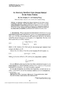
Fig. 1. 2D Model of the FSI Problems
domain, there are two boundary conditions including an outter fluid pressure boundary ∂Ωp subjected to a prescribed pressure, p = p , and a normal pressure boundary ∂Ωz subjected to a prescribed normal pressure gradient nf∇p = w . On the solid domain, there are two boundary conditions including a Neumann boundary ∂Ωu subjected to a prescribed displacements us = u , and a Dirichlet boundary ∂Ωt subjected to prescribed force vectors n s σs = t s . For the present FSI system, the solid is modeled by differential equations of motion of a continuum body subjected to small deformations, while the fluid is modeled by wave equations with small translations and is assumed to be irrotational and inviscid. In addition, the interfacial coupling conditions are used to ensure the compatible displacement and pressure equilibrium between the solid domain and fluid domain. In general, the governing equations and boundary conditions for the present FSI system can be given by (Carlsson, 1992):
(1)
⎧ ∂2 p 2 2 ⎪ -------2- – c0 ∇ p = c20 ∂q -----in Ωf ∂t ⎪ ∂t ⎪ In the fluid domain: ⎨ p = p on ∂Ωp ⎪ on ∂Ωz ⎪ n f∇p = w ⎪ ⎩ + and the initial conditions
(2)
⎧ us n = uf n On the interfacial boundary: ⎨ ⎩ σs n = –p
2. Governing Equations for Analysis of the 2D FSI System In general, a FSI problem can be illustrated by three main components as shown in Fig. 1 which includes a solid domain Ωs, a fluid domain Ωf, and an interfacial boundary between the fluid and solid domain defined by ∂Ωsf = Ωs ∩ Ωf . On the fluid
2 ⎧ T ∂ us in Ωs ⎪ ∇s σs + bs = ρ s --------2 ∂t ⎪ ⎪ In the solid domain: ⎨ us = u on ∂Ωu ⎪ ⎪ n s σs = t s on ∂Ωt ⎪ ⎩ and the initial conditions
on
∂Ωsf
on
∂Ωsf
(3)
in which, for fluid domain p(t) is the dynamic pressure; qf (t) is the added fluid mass per unit volume; c0 is the speed of sound; T 2 2 2 2 2 ∇ = [∂ ⁄ ∂x ∂ ⁄ ∂y ] and ∇ = ∇ ⋅ ∇ = ∂ ⁄ ∂x + ∂ ⁄ ∂y ; and for T solid domain, σ s = [ σ x σ y σ xy ] is the stress vector; us = [usx usy ]T is the displacement vector; bs = [ bsx bsy ]T is the body force
−2−
KSCE Journal of Civil Engineering
An Edge-based Smoothed Finite Element Method (ES-FEM) for Dynamic Analysis of 2D Fluid-Solid Interaction Problems
vector; ρs is the material density; and n f = [ nfx nfy ] is the boundary normal vector pointing outward from the fluid boundary; ∇ s is the 2D symmetric differential operator and ns is the boundary normal matrix pointing outward from the solid boundary defined by: ns = nsx 0 nsy 0 nsy nsx
(4)
In addition in the solid, the kinematic relationship (between displacement vector us and strains εs) and the Hook’s law (between the stresses σs and the strains εs) are given respectively by: εs = ∇s us and σs = Ds εs
Ωf
2 0
2
(6)
Ωf
By using Green-Gauss theorem on the second term, the weak form in Eq. (6) is tranformed into: 2
Ωf
Ωf
∂Ω sf
∂q + c ∫ νf wdS + c ∫ νf -------f dV ∂t ∂Ω z Ωf 2 0
(7)
2 0
Now, by discretizing the fluid domain Ωf into a mesh of Nef three-node triangular elements and Nnf nodes, we can approximate 1 1 the pressure field p ∈ H and the test weight function vf ∈ H0 in the forms of: p = Nf p; νf = Nf cf
T
2 T 2 T ∂q + c0 ∫ Nf wdS + c0 ∫ Nf -------f dΩ ∂t ∂Ωz
or in the matrix form: ·· Mf p + Kf p = f q + fs where, Vol. 00, No. 0 / 000 0000
⎛
2
∂ us⎞
T
(12)
Ωs
By using Green-Gauss theorem and substittuting Eq. (5) on the second term, the weak form in Eq. (12) is tranformed into: ∂ us T T T + ∫ ( ∇svs ) Ds∇ su sdΩ = ∫ vs ns σ sdΓ ∫ vs ρ s ---------dΩ 2 ∂t Ωs Ωs ∂Ωsf T
∂Ωt
u s = N s d s ; vs = N s c s
(10)
(14)
where, ds is the vector containing nodal displacement values; cs is the vector containing nodal chosen test values; and Ns is the vector containing the nodal finite element shape functions. Substituting the approximations us and vs in Eq. (14) into the weak form (13), the finite element formulation for the solid domain is then written as: ·· T T ∫ Ns ρs Ns dΩds + ∫ ( ∇s Ns ) Ds ∇s Ns dΩds Ωs
Ωs
=
∫
N n s σs dΓ + T s
∂Ωsf
s
s
∫
∂Ωt
or in the matrix form: M d·· + K d = f + f s
s
f
T
T
(15)
Ns ts dΓ + ∫ Ns bs dΩ Ωs
(16)
b
where, Ms = ∫ Ns ρ s Ns dΩ; Ks = ∫ ( ∇s Ns ) Ds ∇ s Ns dΩ T
Ωt
T
Ωs
T T ∫ N ns σs dΓ; fb = ∫ Ns tsdΓ + ∫ Ns bs dΩ T s
∂Ωsf
Ωf
Ωs
Now, by discretizing the solid domain Ωs into a mesh of Nes three-node triangular elements and Nns nodes, we can approximate 1 the displacement field u s ∈ H and the test weight function 1 vs ∈ H0 in the forms of:
ff = (9)
(13)
T
+ ∫ vs t sdΓ + ∫ vs bs dΩ
2 2 T T ·· ∫ N Nf dΩp = c0 ∫ ( ∇Nf ) ∇Nf dΩp = c0 ∫ Nf nf ∇pdΓ ∂Ω sf
Ωf
dΩ = 0 ∫ vs ⎝ ∇s σs + b s – ρs --------2 ∂t ⎠
T f
Ωf
∂Ω z
(11)
3.2 Brief on the FEM for Solid Domain (Carlsson, 1992) 1 Let vs ∈ H0 be the test function associated to the solid displacement field us, the weak form corresponding to the first term in Eq. (1) can be obtained by the usual test-function method as:
(8)
where, p is the vector containing the nodal pressure values; cf is the vector containing the nodal chosen test values; and Nf is the vector containing the nodal finite element shape functions. Substituting the approximations p and vf in Eq. (8) into the weak form (7), the finite element formulation for the fluid domain is then written as: Ωf
T 2 T ∂q fq = c ∫ Nf wdΓ + c0 ∫ Nf -------f dΩ ∂t
2
3.1 Brief on the FEM for Fluid Domain (Carlsson, 1992) 1 Let νf ∈ H0 be a test function associated to the pressure field p, the weak form corresponding to the first term in Eq. (2) can be obtained by the usual test-function method as:
∂ p- dV + c2 ( ∇ν )T ∇pdV = c2 ν n ∇pdS 0∫ f 0 ∫ f f ∫ νf ------2 ∂t
Ωf
T f
∂Ωsf
3. ES-FEM for Fluid-Solid Interaction Problems
f⎞ ⎛ ∂ p- – c2∇ 2 p – c2 ∂q 0 0 ------- dV = 0 ∫ νf ⎝ ------2 ∂t ⎠ ∂t
T
2 0
fs = c ∫ N n f∇pdΓ;
(5)
where, Ds ( 3 × 3 ) is a Symmetric Positive Definite (SPD) matrix of material constants.
2
Kf = c0 ∫ ( ∇Nf ) ∇Nf dΩ
T
Mf = ∫ Nf Nf dΩ;
∂Ωt
(17)
∂Ωs
3.3 FEM for the Coupled Fluid - Solid System (Carlsson, 1992) In order to maintain the compatibility and continuity condition on the interface ∂Ωsf between the solid and the fluid, the movement of fluid particles and the solid in the normal direction of the boundary should be identical. To express these conditions,
−3−
T. Nguyen-Thoi, P. Phung-Van, V. Ho-Huu, and L. Le-Anh
we now introduce the vector n = [nx ny ]= [ nfx nfy ]= [–nsx –nsy ] which is the normal vector pointing toward the solid region, and express the continuity of displacement of the two fields in the form of: us ∂Ω = uf ∂Ω or nus = nu f on ∂Ωsf sf
(18)
sf
and the continuity of pressure in the form of: σ s n = n s σs = – p
nsx T =n p nsy
(19)
where, uf = [ufx ufx ]T is the displacement of the fluid particles. Basing on Eq. (19), we now can express the force vector ff in Eq. (17) by the vector of fluid pressure as:
∫ N nsσs dΓ = ∫ N n pdΓ = ∫ N n Nf dΓpf T s
ff =
T s
∂Ωsf
T
T s
T
(20)
∂Ωsf
∂Ωsf
Within the fluid domain, the interactive act is expressed via the force term fs in Eq. (10). By using the relationship between pressure and acceleration in the fluid domain: 2
∂ uf( t ) ∇p = –ρ0 --------------2 ∂t
(21)
and the boundary condition in Eq. (18), we can express the condition n∇p| ∂Ω in the form of: sf
2
2
∂ u f( t ) ∂ us ( t ) n∇ p ∂Ω = –ρ0 n --------------= –ρ 0 n --------------= –ρ 0 nNs d··s ∂Ωsf (22) 2 2 sf ∂t ∂Ω ∂t ∂Ω sf
sf
Then, the force term acting on the fluid fs in Eq. (10), can be described in terms of structural acceleration by: ·· 2 T 2 T 2 T fs = c0 ∫ Nf nf ∇pdΓ = c0 ∫ Nf n∇pdΓ = –ρ 0 c0 ∫ Nf nNsdΓds (23) ∂Ωsf
∂Ωsf
∂Ωsf
Let introduce a spatial coupling matrix as: T T ∫ Ns n NfdΓ
H=
(24)
∂Ωsf
we now can rewrite the coupling forces ff in Eq. (20) and fs in Eq. (23) in the reduced forms as: T 2 f = Hp and f = –c ρ H d·· (25) f
f
s
0
0
s
The coupling fluid-solid interaction problem can be expressed by an unsymmetrical matrix expression as:
2
ρ0 c0 H
d·· s + Ks –H ds = fb 0 Kf pf fq Mf p·· f 0
Ms T
Fig. 2. Mesh of Triangular Elements and the Forming of the Smoothing Cells Associated with Edges in the ES-FEM-T3
the ES-FEM-T3 applies the gradient smoothing technique (Chen ˜ (k) through et al., 2001) to calculate the local stiffness matrix K (k) on the edge-based smoothing cells Ω which are created by connecting two endpoints of the edge to centroids of contiguous elements as shown in Fig. 2. 3.4.1 ES-FEM-T3 for the Fluid Domain in the Coupled Fluid - Solid System Based on the triangular discretization generated in the standard (k ) FEM-T3, a smoothing cell Ωf in the ES-FEM-T3 is created by connecting two end-points of edge k with centroids of the contiguous triangles sharing the edge k. With such the manner, ed the fluid domain can be further divided into Nf smoothing N (k ) (k) ( i) ( j) cells Ωf such that, Ωf = ∪ Ωf , Ωf ∩ Ωf = ∅ , i ≠ j , where k=1 ed N f is the total number of edges of the finite element mesh. Now by using the gradient smoothing technique (Chen et al., 2001), the pressure gradient ∇p in Eq. (9) can be used to ˜ p(k) on the smoothing define the smoothed pressure gradient ∇ (k) cell Ωf as: ˜ p(k) = ∇pΦ(k )( x )dΩ ∇ (27) ed f
∫
f
( k)
Ωf (k)
where, Φf ( x ) is a given smoothing function which satisfies at least the unity property ∫Ω Φ(f k) ( x )dΩ = 1 . Normally, the following Heaviside constant smoothing function fitting this property is used in the ES-FEM (k ) f
(k )
⎧ 1 ⁄ Af (k) Φf ( x ) = ⎨ ⎩ 0
(26)
(k)
x ∈ Ωf
(28)
(k)
x ∉ Ωf
(k)
3.4 Edge-based Smoothed Finite Element Method using Triangular Elements (ES-FEM-T3) Basically, the ES-FEM-T3 inherited all the fundamental properties of FEM-T3 using triangular elements including the triangular mesh discretization, the linear nodal shape functions and continuous approximated fields (displacement or pressure) on the whole problem domain. However, unlike the standard FEM-T3 which calculates the local stiffness matrix Ke through on the elements,
where, A(f k) = ∫Ω dΩ is the area of the smoothing cell Ωf . Next by applying a divergence theory, we acquire the constant ˜ p(k ) over the domain Ω(k) as smoothed pressure gradient ∇ f following: ( k) f
˜ p( k ) = ∇
∑ B˜ fI( xk )pI
(29)
(k )
I ∈ Nf (k) f
where, N is the total number of nodes of elements containing (k) (k) the common edge k ( Nf = 3 for boundary edges and Nf = 4 for
−4−
KSCE Journal of Civil Engineering
An Edge-based Smoothed Finite Element Method (ES-FEM) for Dynamic Analysis of 2D Fluid-Solid Interaction Problems
˜ fI ( x ) is denoted as the inner edges as shown in Fig. 2), and B k (k) smoothed pressure gradient matrix on the smoothing cell Ωf , ˜ ˜ fI( x ) = bfIx( x k ) B k b˜ fIy( x k )
˜ sI ( x ) = B k
(30)
(k ) 1 b˜ fIx ( x k ) = ------- NfI ( x )nfx ( x )dΓ, (k) ∫ Af Γ (k) f
(k ) 1 b˜ sIx ( x k ) = ------- N sI( x )nsx ( x )dΓ, (k) ∫ As Γ (k ) s
(31)
(k ) 1 - NfI ( x )nfy ( x )dΓ b˜ fIy ( x k ) = ------(k) ∫ Af Γ
(k ) 1 - N sI( x )nsy ( x )dΓ b˜ xIy ( xk ) = ------(k ) ∫ As Γ
(k)
where, nfx and nfy are two components of the outward normal (k) vector on the boundary Γf . Next, by using the same assembly manner as in the FEM, the ˜ can be expressed by: global smoothed stiffness matrix K f ed
ed
(k ) ∑ K˜ fIJ
2˜T ˜ (k) ˜T ˜ ∫ BfIBfJ dΩ = c0 BfIBfIAf
˜ where, K by: k) ˜ (sIJ K =
(33)
ed s
(34)
(39)
is the edge-based smoothed stiffness matrix computed
˜ ˜ ˜ ˜ (k) ∫ BsIDBsJdΩ = BsIDBsJ As T
T
(40)
( k) Ωs
(k) Ωf
3.4.2 ES-FEM-T3 for the Solid Domain in the Coupled Fluid - Solid System Similarly to the fluid domain, the solid domain is also divided N ed (k) into Ns smoothing cells Ωs such that Ωs = ∪ Ω(sk) and k=1 ( i) (j) ed Ωs ∩ Ωs = ∅ , i ≠ j , where N s is the total number of edges of the finite element mesh in the solid domain. And then by using the gradient smoothing technique (Chen et al., 2001), the compatible displacement gradient ∇s us in Eq. (13) is used to define the smoothed displacement gradient ∇su s on the smoothing cell Ω(sk) as:
(k)
∑ K˜ sIJ
k=1 (k) sIJ
k=1
˜ (fIJk) is the edge-based smoothed stiffness matrix computed where, K by:
Ns
˜s= K
(32)
˜ su( k) ( x ) = ∇ u ( x )Φ(k ) ( x )dΩ ∇ s s ∫ s s
(38)
where, n(sxk) and n(syk) are two components of the outward normal (k) vector on the boundary Γs . Next, by using the same assembly manner as in the FEM, the ˜ can be expressed by: global smoothed stiffness matrix K s
Nf
˜ (fIJk) = c2 K 0
(37)
( k) s
(k) f
˜f= K
0 ˜ 0 bsIy( xk ) ˜bsIy ( x ) b˜ sIx( x ) k k
in which, the non-zero items are calculated by:
and its items are computed by:
(k )
b˜ sIx( xk )
3.5 ES-FEM-T3 for 2D Fluid - Solid Interaction Problems As presented in section 3.4, two basic differences between the ES-FEM-T3 and the FEM-T3 is the way to define the gradient fields and the way to compute the stiffness matrix. In the FEMT3, the compatible gradient fields on the elements are used and the stiffness matrices Kf and Ks are calculated based on the elements. While in the ES-FEM-T3, the smoothed gradient fields on the edge-based smoothing domains are used and the ˜ are calculated based on ˜ and K smoothed stiffness matrices K s f the edge-based smoothing domains. Therefore based on Eq. (26), the global system of equations for the fluid–solid interaction problems using the ES-FEM-T3 can be expressed in the form of:
(k)
Ωs
where, Φ(sk ) ( x ) is the constant Heaviside smoothing function defined as: (k)
(k)
⎧ 1 ⁄ As (k ) Φs ( x ) = ⎨ ⎩ 0
x ∈ Ωs
(k )
x ∉ Ωs
(35)
where, A(sk) = ∫ dΩ is the area of the cell Ω(sk) . Ω Next by applying a divergence theory, we acquire the constant smoothed displacement gradient ∇˜ su (sk ) over the domain Ω(sk) as following: ˜ s u(k) = ˜ sI( x )d ∇ B (36) (k) s
s
∑
( k)
k
I
I ∈ Ns
where, N(sk) is the total number of nodes of elements sharing the edge k, and B˜ sI( xk ) is denoted as the smoothed displacement gradient matrix on the smoothing cell Ω(sk) , Vol. 00, No. 0 / 000 0000
˜ 0 d··s K + s – H d s = fb (41) ˜ f pf fq ρ c H Mf p·· f 0 K ˜ and K ˜ are calculated by Eqs. (39) and (32), where, K s f respectively. Ms
2 0 0
T
4. Dynamic Analysis Stability is a one of the primary concerns in dynamic analysis. On this aspect, the ES-FEM-T3 shows the excellent properties in both spacially and temporally stable (Liu and Nguyen-Thoi, 2010; Liu et al., 2009b). Hence, it is very suitable to apply the ES-FEM-T3 for free and forced vibration analyses of the fluidsolid interaction problems. For the case of considering the damping forces, Eq. (41) for the dynamic anlysis of the fluid– solid interaction problems using the ES-FEM-T3 can be
−5−
T. Nguyen-Thoi, P. Phung-Van, V. Ho-Huu, and L. Le-Anh
described as: ˜ x + Cx· + Mx·· = F K
(42)
where, x=
˜ s –H Ms ˜ = K ;K ;M= 2 T ˜ pf ρ 0 c0 H 0 Kf
ds
0 Mf
; F = fb (43) fq
and C is the Rayleigh damping matrix assumed to be propotional ˜ and the mass matrix M as: to both the stiffness matrix K ˜ C = αM + βK
(44)
where, α and β are the Rayleigh damping coefficients. To solve the second-order time dependent problem Eq. (42), the Newmark method is employed in this paper. The basic procedure of this direct integration method is to sub-divide the reponse period T into n intervals of length ∆t = T/n and then to determine the solution of the equibrilium equation at each step. In detail, at the interval t = t0, the initial state ( x0, x· 0, x··0 ) is assumed known. Then our aim is to find a new state ( x1, x· 1, x··1 ) at the next interval t1 = t0 + θ∆t where. The process can be described by the following equations: 1 ⎞ ˜ x = θ∆tF + ( 1 – θ )∆tF ⎛ α + -------M + ( β + θ∆t )K 1 1 0 ⎝ θ∆t⎠
Fig. 4. Mesh using Triangular Elements for both Fluid and Solid Domains of the 2D Deformable Solid Attached with a Closed Tank Filled with Water
(45)
1 1 ˜x + ⎛ α + --------⎞ Mx0 + --- Mx· 0 + [β – ( 1 – θ ) ∆t ]K 0 ⎝ θ ∆t⎠ θ
1 1–θ x· 1 = -------- ( x 1 – x 0 ) – ----------x· 0 θ ∆t θ
(46)
1 1–θ x··1 = -------- ( x· 1 – x· 0 ) – ----------x··0 θ ∆t θ
(47)
In the case the damping and forcing terms are ignored, Eq. (42) is reduced into a homogenous differential equation by: ˜ x + Mx·· = 0 K
Fig. 3. Model of a 2D Deformable Solid Backed by a Closed Tank Filled with Water
(48)
5.1 Dynamic Analysis of a 2D Deformable Solid Backed by a Closed Box Filled with Water In this example, we analyze a clamped 2D deformable solid backed by a closed rectangular tank filled with water as shown in Fig. 3. The dimension of the rectangular tank is given by 10 m × 4 m. The data of the fluid in the tank is given by the fluid material density ρ = 1000 kg/m2 and speed of air c = 1500 m/s2, and the data of the solid is given by the material density ρs = 2500 kg/m2, elastic module E = 2.1 × 10⁹ N/m2 and poisson’s ratio υ = 0.3. The model is discretized by a mesh of triangular elements for
and the corresponding eigenvalue equation of Eq. (48) is written in the form of: 2
˜ – ω M]x = 0 [K
(49)
where, ω is the angular frequency and x is the amplitude of the sinusoidal displacements expressed by x = xexp ( iωt ) .
5. Numerical Examples This section presents two numerical examples to demonstrate the superior features of the ES-FEM-T3 in analysing the dynamic behaviours of the coupled fluid-solid interaction problems. The accuracy and stability of ES-FEM-T3 will be verified by comparing its numerical results with those of standard FEM-T3 and FEM-Q4 using four-node elements. Moreover, the numerical solutions by FEM-Q8 using 8-node elements will be used as the reference solutions for convergence analysis of the numerical methods.
Fig. 5. Comparison on the Convergence of the First Coupled Eigenmode by Three Methods: ES-FEM-T3, FEM-T3 and FEMQ4
−6−
KSCE Journal of Civil Engineering
An Edge-based Smoothed Finite Element Method (ES-FEM) for Dynamic Analysis of 2D Fluid-Solid Interaction Problems
both fluid and solid domains as shown in Fig. 4. 5.1.1 Free Vibration Analysis At first, we conduct an eigenmode analysis to determine the frequencies and natural mode shapes of the fluid solid system. The result by the FEM-Q8 with 1290 DOFs for solid and 729 Degree Of Freedom (DOFs) for fluid is chosen as the reference solution. This choice is rational because it is not only consistent with those of the comsol solution but also reflects the mesh quality (high-order element) required in conventional FEM in order to achieve close-to-exact solutions. Three different coupled methods: the FEM-T3, FEM-Q4 and ES-FEM-T3 using the same set of DOFs are investigated for the benchmarking. Fig. 5 compares the convergence of the first eigenmode obtained from the testing methods. It can be seen that the ES-FEM-T3 acquired the best results and even performed much better than the FEMQ4 using bilinear elements. Frequencies of seven coupled eigenmodes by the testing methods are presented in Fig. 6. The results again show that the
ES-FEM-T3 is closest to both the reference solution and the comsol solution. In addition, Fig. 7 illustrates the value and shape of first nine coupled eigenmodes obtained from the ESFEM-T3. It is observed that the shapes express correctly the real physical vibration modes of the system without spurious nonzero energy mode. 5.1.2 Forced Vibration Analysis In this example, we study the dynamic response of the FSI system by the ES-FEM-T3. The applied force is a harmonic vertical load F ( x, ω ) = δc ( x)iωeiωt at point x, where δc ( x ) is the Dirac function. First, we consider the case t = 0 where the point x is set up at point A (2.0, 5.0) as in Fig. 4. The temporal frequency ω /2π is adjusted in the distance from 3 Hz to 17 Hz covering the scope of the first three coupled eigenfrequencies of the system given in Fig. 7. Fig. 8 shows the corresponding displacement responses measured at the loading point A(2.0, 5.0). The results show that the peaks of the first three modes happen when the force frequency reaches the first three eigenfrequencies. Keeping the same context, we change the loading point position to point B(2.0, 3.0) and still measure the displacement responses at the
Fig. 6. Comparison on Seven Coupled Eigenmodes of the FSI System by Three Methods: ES-FEM-T3, FEM-T3 and FEM-Q4 Fig. 8. Displacement Response at Point A(2.0, 5.0) by the ES-FEMT3 (for the case the force applied also at point A(2.0, 5.0))
Fig. 7. Mode Shapes Corresponding to 9 Coupled Eigenmodes of the FSI System by the ES-FEM-T3 Vol. 00, No. 0 / 000 0000
Fig. 9. Displacement Response at Point A(2.0, 5.0) by the ESFEM-T3 (for the case the force applied to point B(2.0, 3.0))
−7−
T. Nguyen-Thoi, P. Phung-Van, V. Ho-Huu, and L. Le-Anh
Table 1. Comparison on Values of Seven First Coupled and Uncoupled Eigenmodes of Solid Method Without coupling With coupling
1 3.0511 5.4897
2 7.8045 10.4565
Mode sequence number 3 4 14.0971 15.3153 15.2791 17.8334
Fig. 10. Comparison of Displacement Response at Point A(2.0, 5.0) by ES-FEM-T3 under Coupling and Uncoupling Conditions
Fig. 11. Comparison of the Displacement Response at Point A(2.0, 5.0) between the ES-FEM-T3 and FEM-Q4 (for the case the force applied also at point A(2.0, 5.0))
point A(2.0, 5.0) as shown in Fig. 9. The results again show that the peak values happen exactly at the first three eigenfrequencies. To that extent, the ES-FEM-T3 method illustrates the ability to produce adequate details for the modal analysis and dynamic analysis of the fluid-solid interaction system. Moreover, the forced frequency response analysis also provides different eigenfrequencies of the solid system under coupling and uncoupling conditions. As seen in Table 1 and Fig. 10, the eigenfrequency values of the coupling fluid-solid system are much greater than those of the uncoupling solid system. Therefore, it is essential to employ the fluid-solid interaction model for correct simulation of the behaviour of the solid system coupling with the fluid.
5 21.4347 24.8878
6 29.5174 30.4727
7 30.5690 33.8092
Fig. 12. Comparison of the Displacement Response at Point A(2.0, 5.0) by ES-FEM-T3, FEM-T3 and FEM-Q4 (for the case the force applied also at point A(2.0, 5.0))
The accuracy of the ES-FEM-T3 in the dynamic response analysis of the FSI system is also demonstrated by comparing its displacement responses with those from the FEM-Q4 and the reference solution as shown in Fig. 11. It is clear that the ESFEM-T3 provides the closest results to the reference solution by the FEM-Q8. Moreover, Fig. 11 also illustrates the increasing trend of the deviation between the testing methods versus the reference solution as the frequency increases. Both the ES-FEMT3 and the FEM-Q4 follow this trend, however, the variance of the ES-FEM-T3 are much smaller than those of the FEM-Q4. Fig. 12 presents the transient response by the ES-FEM-T3 and the FEM-Q4. It also exhibits that the displacement responses by the ES-FEM-T3 are closer to those by the reference solution. Through the example, the accurate and robust performance of the ES-FEM-T3 for dynamic analysis of the FSI system is mainly verified by comparing its eigenfrequencies, frequency responses and transient responses with those of other standard FEM models.
−8−
Fig. 13. 2D Model of a Deformable Water Dam KSCE Journal of Civil Engineering
An Edge-based Smoothed Finite Element Method (ES-FEM) for Dynamic Analysis of 2D Fluid-Solid Interaction Problems
method, both the displacement in the solid domain and the pressure in the fluid domain are smoothed by the gradient smoothing technique based on the smoothing domains associated with the edges of triangular elements. The edge-based smoothing technique takes advantage from generating the triangular elements for complex geometry domains and the soften effect by the gradient smoothing technique to relieve the overstiff behavior of the standard FEM-T3. Through some numerical examples for dynamic analysis of the FSI problems, it is seen that the ES-FEM-T3 shows the outstanding performance in eigenfrequencies, frequency responses and transient responses compared to some existing FEM models.
Fig. 14. Mesh using Triangular Elements for the FSI System
Acknowledgements This work was supported by Vietnam National Foundation for Science & Technology Development (NAFOSTED), Ministry of Science & Technology, under the basic research program for the author T. Nguyen-Thoi.
References
Fig. 15. Comparison on Convergence of the First Coupled Eigenmode by Three Methods: ES-FEM-T3, FEM-T3 and FEM-Q4
5.2 2D Deformable Water Dam In this example, we investigate an eigenmode analysis for a 2D model of the deformable water dam with fixed foundation as shown in Fig. 13. Data of the dam is given by the solid material density ρs = 2500 kg/m2, elastic module E = 2.1 × 10⁹ N/m2 and poisson’s ratio υ = 0.3. The water is blocked by the dam and filled up to the dimension of 10m × 4m. Data of the water is given by density ρ = 1000 kg/m2 and speed of air c = 1500 m/s2. The model is discretized by a mesh of triangular elements for both fluid and solid domains as shown in Fig. 14. Similarly to the previous example, the reference solution is also computed by the FEM-Q8 with 697 Degree Of Freedom (DOFs) for the fluid domain and 1570 DOFs for the solid domain. Three coupled methods are employed for the benchmarking are the FEM-T3, FEM-Q4 and ES-FEM-T3. Convergent rates of the first eigenmode obtained by the testing methods are shown in Fig. 15. The results again comfirm the outstanding performance of the ES-FEM-T3 compared with the FEM-Q4 and FEM-T3 for eigenmode analysis of FSI problems.
6. Conclusions This paper further extends the application of the ES-FEM-T3 to the dynamic analyses of the 2D fluid-solid interaction problems based on the pressure-displacement formulas. In the proposed Vol. 00, No. 0 / 000 0000
Bathe, K. J., Nitikitpaiboon, C., and Wang, X. (1995). “A mixed displacement-based finite element formulation for acoustic fluidstructure interaction.” Computers and Structures, Vol. 56, Nos. 2-3, pp. 225-237. Brunner, D., Junge, M., and Gaul, L. (2009). “A comparison of FE–BE coupling schemes for large-scale problems with fluid–structure interaction.” International Journal for Numerical Methods in Engineering, Vol. 77, No. 5, pp. 664-688. Carlsson, H. (1992). Finite element analysis of structure-acoustic systems; formulations and solution strategies, PhD Thesis, Lund University, Lund, Sweden. Chen, H. C. and Taylor, R. L. (1990). “Vibration analysis of fluid-solid systems using a finite element displacement formulation.” International Journal for Numerical Methods in Engineering, Vol. 29, No. 4, pp. 683-698. Chen, J. S., Wu, C. T., Yoon, S., and You, Y. (2001). “A stabilized conforming nodal integration for Galerkin mesh-free methods.” International Journal for Numerical Methods in Engineering, Vol. 50, No. 2, pp. 435-466. Dai, K. Y., Liu, G. R., and Nguyen, T. T. (2007). “An n-sided polygonal Smoothed Finite Element Method (nSFEM) for solid mechanics.” Finite Elements in Analysis and Design, Vol. 43, Nos. 11-12, pp. 847-860. Everstine, G. C. and Henderson, F. M. (1990). “Coupled finite element/ boundary element approach for fluid structure interaction.” The Journal of the Acoustical Society of America, Vol. 87, No. 5, pp. 1938-1947. He, Z. C., Liu, G. R., Zhong, Z. H., Zhang, G. Y., and Cheng, A. G. (2010). “Coupled analysis of 3D structural–acoustic problems using the edge-based smoothed finite element method/finite element method.” Finite Elements in Analysis and Design, Vol. 46, No.12, pp. 1114-1121. Liu, G. R., Dai, K. Y., and Nguyen-Thoi, T. (2007a). “A smoothed finite element method for mechanics problems.” Computational Mechanics, Vol. 39, No. 6, pp. 859-877. Liu, G. R., Nguyen-Thoi, T., Dai, K. Y., and Lam, K. Y. (2007b). “Theoretical aspects of the Smoothed Finite Element Method
−9−
T. Nguyen-Thoi, P. Phung-Van, V. Ho-Huu, and L. Le-Anh
(SFEM).” International Journal for Numerical Methods in Engineering; Vol. 71, No. 8, pp. 902-930. Liu, G. R., Nguyen-Thoi, T., Nguyen-Xuan, H., and Lam, K. Y. (2009a). “A Node based Smoothed Finite Element Method (NS-FEM) for upper bound solution to solid mechanics problems.” Computers and Structures, Vol. 87, Nos. 1-2, pp. 14-26. Liu, G. R., Nguyen-Thoi, T., and Lam, K. Y. (2009b). “An Edge-based Smoothed Finite Element Method (ES-FEM) for static, free and forced vibration analyses of solids.” Journal of Sound and Vibration, Vol. 320, Nos. 4-5, pp. 1100-1130. Liu, G. R., Nguyen-Thoi, T., Nguyen-Xuan, H., Dai, K. Y., and Lam, K. Y. (2009c). “On the essence and the evaluation of the shape functions for the Smoothed Finite Element Method (SFEM)” International Journal for Numerical Methods in Engineering, Vol. 77, No. 13, pp. 1863-1869. Liu, G. R. and Nguyen-Thoi, T. (2010). Smoothed finite element methods, CRC Press, Taylor and Francis Group, NewYork. Liu, G. R., Nguyen-Xuan, H., and Nguyen-Thoi, T. (2010a). “A theoretical study on the Smoothed FEM (S-FEM) models: Properties, accuracy and convergence rates.” International Journal for Numerical Methods in Engineering, Vol. 84, No. 10, pp. 1222-1256. Liu, G. R., Chen, L., Nguyen-Thoi, T., Zeng, K., and Zhang, G. Y. (2010b). “A novel singular node-based smoothed finite element method (NSFEM) for upper bound solutions of cracks.” International Journal for Numerical Methods in Engineering, Vol. 83, No. 11, pp. 1466-1497. Luong-Van, H., Nguyen-Thoi, T., Liu, G. R., and Phung-Van, P. (2013). “A Cell-based smoothed Finite Element Method using Mindlin plate element (CS-FEM-MIN3) for dynamic response of composite plates on viscoelastic foundation.” Engineering Analysis with Boundary Elements, Vol. 42, pp. 8-19. Nguyen-Thoi, T., Liu, G. R., Dai, K. Y., and Lam, K. Y. (2007). “Selective smoothed finite element method.” Tsinghua Science and Technology, Vol. 12, No. 5, pp. 497-508. Nguyen-Thoi, T., Liu, G. R., and Nguyen-Xuan, H. (2009a). “Additional properties of the Node-based Smoothed Finite Element Method (NS-FEM) for solid mechanics problems.” International Journal of Computational Methods, Vol. 6, No. 4, pp. 633-666. Nguyen-Thoi, T., Liu, G. R., Vu-Do, H. C., and Nguyen-Xuan, H. (2009b). “An Edge–based Smoothed Finite Element Method (ESFEM) for visco-elastoplastic analyses of 2D solids using triangular mesh.” Computational Mechanics, Vol. 45, No. 1, pp. 23-44. Nguyen-Thoi, T., Liu, G. R., Lam, K. Y., and Zhang, G. Y. (2009c). “A Face-based Smoothed Finite Element Method (FS-FEM) for 3D linear and nonlinear solid mechanics problems using 4-node tetrahedral elements.” International Journal for Numerical Methods in Engineering, Vol. 78, No. 3, pp. 324-353. Nguyen-Thoi, T., Vu-Do, H. C., Rabczuk, T., and Nguyen-Xuan, H. (2010a). “A Node-based Smoothed Finite Element Method (NS-FEM) for upper bound solution to visco-elastoplastic analyses of solids using triangular and tetrahedral meshes.” Computer Methods in Applied Mechanics and Engineering, Vol. 199, Nos. 45-48, pp. 3005-3027. Nguyen-Thoi, T., Liu, G. R., and Nguyen-Xuan, H. (2010b). “An nsided polygonal Edge-based Smoothed Finite Element Method (nES-FEM) for solid mechanics.” Communications in Numerical Methods in Engineering, Vol. 27, No. 9, pp. 1446-1472. Nguyen-Thoi, T., Phung-Van, P., Nguyen-Xuan, H., and Thai-Hoang, C. (2012). “A cell-based smoothed discrete shear gap method using triangular elements for static and free vibration analyses of Reissner– Mindlin plates.” International Journal for Numerical Methods in Engineering; Vol. 91, No. 7, pp. 705-741.
Nguyen-Thoi, T., Phung-Van, P., Luong-Van, H., Nguyen-Van, H., and Nguyen-Xuan, H. (2013a). “A Cell-Based smoothed three-node Mindlin plate element (CS-MIN3) for static and free vibration analyses of plates.” Computational Mechanics, Vol. 50, No. 1, pp. 65-81. Nguyen-Thoi, T., Bui-Xuan, T., Phung-Van, P., Nguyen-Xuan, H., and Ngo-Thanh, P. (2013b). “Static, free vibration and buckling analyses of stiffened plates by CS-FEM-DSG3 using triangular elements.” Computers & Structures, Vol. 125, pp. 100-113. Nguyen-Thoi, T., Phung-Van, P., Thai-Hoang, C., and Nguyen-Xuan, H. (2013c). “A Cell-based Smoothed Discrete Shear Gap method (CSFEM-DSG3) using triangular elements for static and free vibration analyses of shell structures.” International Journal of Mechanical Sciences, Vol. 74, pp. 32-45. Nguyen-Thoi, T., Phung-Van, P., Nguyen-Hoang, S., and Lieu-Xuan, Q. (2014). “A smoothed coupled NS/nES-FEM for dynamic analysis of 2D fluid-solid interaction problems.” Applied Mathematics and Computation, Vol. 232, pp. 324-346. Nguyen-Xuan, H., Liu, G. R., Nguyen-Thoi, T., and Nguyen-Tran, C. (2009a). “An Edge–based Smoothed Finite Element Method (ESFEM) for analysis of two–dimensional piezoelectric structures.” Smart Materials and Structures, Vol. 18, No. 6, pp. 065015. Nguyen-Xuan, H., Liu, G. R., Thai-Hoang, C., and Nguyen-Thoi, T. (2009b). “An edge-based smoothed finite element method with stabilized discrete shear gap technique for analysis of ReissnerMindlin plates.” Computer Methods in Applied Mechanics and Engineering, Vol. 199, Nos. 9-12, pp. 471-489. Nguyen-Xuan, H., Tran, L. V., Thai, C. H., and Nguyen-Thoi, T. (2012). “Analysis of functionally graded plates by an efficient finite element method with node-based strain smoothing.” Thin-Walled Structures, Vol. 54, pp. 1-18. Phung-Van, P., Nguyen-Thoi, T., Tran, V. Loc, and Nguyen-Xuan, H. (2013a). “A Cell-based Smoothed Discrete Shear Gap Method (CSFEM-DSG3) based on the C0-type higher-order shear deformation theory for static and free vibration analyses of functionally graded plates.” Computational Materials Science, Vol. 79, pp. 857-872. Phung-Van, P., Nguyen-Thoi, T., Le-Dinh, T., and Nguyen-Xuan, H. (2013b). “Static, free vibration analyses and dynamic control of composite plates integrated with piezoelectric sensors and actuators by the Cell-based Smoothed Discrete Shear Gap Method (CS-FEMDSG3).” Smart Materials and Structures, Vol. 22, No. 9. Rabczuk, T., Gracie, R., Song, J. H., and Belytschko, T. (2010). “Immersed particle method for fluid-structure interaction.” International Journal for Numerical Methods in Engineering, Vol. 81, No. 1, pp. 48-71. Smith, I. M. and Griffiths, D. V. (1998). Programming the finite element method, Third Ed. Wiley, New York. Thai, H. C., Tran, V. L., Tran, T. D., Nguyen-Thoi, T., and NguyenXuan, H. (2012). “Analysis of laminated composite plates using higher-order shear deformation plate theory and node-based smoothed discrete shear gap method.” Applied Mathematical Modelling, Vol. 36, No. 11, pp. 5657-5677. Wall, W. A. and Rabczuk, T. (2008). “Fluid-structure interaction in lower airways of CT-based lung geometries.” International Journal for Numerical Methods in Fluids, Vol. 57, No. 5, pp. 653-675. Wang, X. D. and Bathe, K. J. (1997). “Displacement pressure based mixed finite element formulations for acoustic fluid–structure interaction problems.” International Journal for Numerical Methods in Engineering, Vol. 40, No. 11, pp. 2001-2017. Wilson, E. L. and Khalvati, M. (1983). “Finite elements for the dynamic analysis of fluid-solid systems.” International Journal for Numerical Methods in Engineering; Vol. 19, No. 11, pp. 1657-1668.
− 10 −
KSCE Journal of Civil Engineering