780â785, 1997. [2] K. Toyama, J. Krumm, B. Brumitt, and B. Meyers, âWallflower: Prin- ciples and practice of background maintenance,â in International Con-.
AN EFFICIENT AND ROBUST SEQUENTIAL ALGORITHM FOR BACKGROUND ESTIMATION IN VIDEO SURVEILLANCE Vikas Reddy ,†‡ Conrad Sanderson ,†‡ Brian C. Lovell †‡ NICTA, PO Box 6020, St Lucia, QLD 4067, Australia ∗ The University of Queensland, School of ITEE, QLD 4072, Australia †
‡
ABSTRACT Many computer vision algorithms such as object tracking and event detection assume that a background model of the scene under analysis is known. However, in many practical circumstances it is unavailable and must be estimated from cluttered image sequences. We propose a sequential technique for background estimation in such conditions, with low computational and memory requirements. The first stage is somewhat similar to that of the recently proposed agglomerative clustering background estimation method, where image sequences are analysed on a patch by patch basis. For each patch location a representative set is maintained which contains distinct patches obtained along its temporal line. The novelties lie in iteratively filling in background areas by selecting the most appropriate candidate patches according to the combined frequency responses of extended versions of the candidate patch and its neighbourhood. It is assumed that the most appropriate patch results in the smoothest response, indirectly enforcing the spatial continuity of structures within a scene. Experiments on real-life surveillance videos demonstrate the efficacy of the proposed method. 1. INTRODUCTION Real-time segmentation, tracking and analysis of foreground objects of interest are fundamental tasks within the area of intelligent video surveillance. Many approaches for detecting and tracking objects are based on background subtraction, where each frame is compared against a background model. The majority of the background subtraction methods described in the literature (e.g. [1, 2, 3]) adaptively model and update the background for every new input frame. However, most of them presume the training image sequence used to model the background is free from foreground objects. This assumption rarely holds true in uncontrolled environments such as train stations and motorways, where directly obtaining a clear background is almost impossible. Furthermore, in outdoor video surveillance a strong illumination change can render the existing background model ineffective. In such circumstances, it becomes inevitable to estimate the background using cluttered sequences (i.e. where parts of the background are occluded). Existing methods to address this problem can be broadly classified into three categories: (i) pixel-level processing, (ii) region-level processing, and (iii) a hybrid of the above methods. For pixel-level processing, the simplest techniques are based on applying a median filter on pixels at each location across all the frames. A background pixel is estimated correctly if it is exposed for more than 50% of the time — often a strong assumption. In [4], the algorithm finds pixel ∗ NICTA is funded by the Australian Government via the Department of Broadband, Communications and the Digital Economy, as well as the Australian Research Council through the ICT Centre of Excellence program.
978-1-4244-5654-3/09/$26.00 ©2009 IEEE
1109
intervals of stable intensity in the image sequence, then heuristically chooses the value of the longest stable interval to most likely represent the background. In [5], an algorithm based on a Bayes’ theorem is proposed. For every new pixel it estimates the intensity value to which that pixel has the maximum posterior probability. In [6], the first stage is similar to that of [4], followed by choosing background pixel values whose interval maximises an objective function. Pixelbased methods are fast but they do not take spatial relationships between pixels into account. This leads to poor background estimation in cluttered or crowded scenes — a problem that can be alleviated by region-level methods. Under region-level processing, the method proposed in [7] roughly segments input frames into foreground and background regions by working on patches. In [8] an algorithm based on agglomerative clustering is presented, where patches are clustered along their time-line, followed by incrementally estimating the background using principles of visual grouping. The algorithm presented in [9] is in the hybrid category. The first stage is similar to that of [4], with the second stage estimating the likelihood of background visibility by computing the optical flow of patches between successive frames. These methods perform well when foreground objects are always moving but tend to fail if the objects move slowly or are quasistationary for extended periods. In this paper we propose an algorithm that addresses these problems and has computational as well as practical advantages. It falls into the region-level category, with its first stage being similar to that of [8]. Specifically, image sequences are analysed on a patch by patch basis. For each patch location a representative set is maintained which contains distinct patches obtained along its temporal line. The novelties of the proposed algorithm are as follows. Unlike the abovementioned techniques, it does not expect all frames of the sequence to be stored in memory simultaneously — instead, it processes the frames sequentially. Background areas are iteratively filled by selecting the most appropriate candidate patches according to the combined frequency responses of extended versions of the candidate patch and its neighbourhood. It is assumed that the most appropriate patch results in the smoothest response, indirectly exploiting the spatial correlations within small regions of a scene. We continue as follows. Section 2 describes the proposed algorithm in detail. Results from experiments on real-life surveillance videos are summarised in Section 3, followed by the main findings in Section 4. 2. PROPOSED ALGORITHM We first provide an overview of the proposed algorithm, followed by a description of its components (Sections 2.1 to 2.3). The algorithm has three stages.
ICIP 2009
(i) (ii) (iii) (iv) (v) Fig. 1: (i) Example frame from an image sequence, (ii) initial background, (iii) iteration 75, (iv) iteration 120, (v) reconstructed background.
Let the resolution of the greyscale image sequence I be W × H. In the first stage, each frame is divided into blocks (patches) of size N × N pixels. Let If be the f -th frame of the training image sequence and let its blocks be denoted by Bf (i, j), for i = 0, 1, 2, · · · , (W/N ) − 1, j = 0, 1, 2, · · · , (H/N ) − 1 and f = 1, 2, · · · , F , where F is the total number of frames. For convenience, each block Bf (i, j) is vectorised into an N 2 dimensional vector bf (i, j). For each block location (i, j), a representative set R(i, j) is maintained. It contains only unique representative blocks, rk (i, j) for k = 1, 2, . . . , S (with S ≤ F ) that were obtained along its temporal line. To determine uniqueness, the similarity of blocks is calculated as described in Section 2.1. Let Wk denote the number of occurrences of rk in the sequence, i.e., the number of blocks at location (i, j) which are deemed to be the same as rk (i, j). It is assumed that one element of R(i, j) corresponds to the background block. To ensure blocks from moving objects are not stored, block bf (i, j) will be registered as rk+1 (i, j) only if it appears in at least two consecutive frames. In the second stage, representative sets R(i, j) having just one block are considered to initialise the corresponding block locations BG(i, j) in the background BG. In the third stage, an empty background block is selected and filled with a block from the corresponding representative set R(i, j). The procedure for selecting the location of an empty background block is described in Section 2.2. Each representative block rk (i, j) is analysed (along with its already filled neighbourhood) in the frequency domain. The details of the analysis and the selection of the most appropriate representative block is described in Section 2.3. The overall pseudo-code of the algorithm is given in Listing 1 and an example of the algorithm in action is shown in Fig. 1.
Stage 1 - Collection of block representatives 1. R ← ∅ (null set) 2. for f = 1 to F do (a) Split input frame If into blocks, each with a size of N × N . (b) for each block Bf (i, j): i. Vectorise block Bf (i, j) into bf (i, j). ii. Find the representative block rm (i, j) from the set R(i, j) = (rk (i, j)|1 ≤ k ≤ S), matching to bf (i, j) based on conditions in Eqns. (1) and (2). if (R(i, j) = {∅} or there is no match) then k ← k + 1. Add a new representative block rk (i, j) ← bf (i, j) to set R(i, j) and initialise its weight, Wk (i, j), to 1. else Update the matched block rm (i, j) and its weight Wm (i, j) as: (r
end if
(i,j)W
(i,j)+b (i,j))
m f rm (i, j) ← m Wm (i,j)+1 Wm (i, j) ← Wm (i, j) + 1
end for each end for Stage 2 - Partial background reconstruction 1. BG ← ∅ 2. for each set R (i, j) if (size(R (i, j)) = 1) then BG (i, j) ← r1 (i, j) . end if end for each
2.1. Similarity Criteria for Blocks We assert that two blocks bf (i, j) and rk (i, j) are similar if the following two constraints are satisfied: � �� � (rk (i, j) − μrk (i, j))� bf (i, j) − μbf (i, j) / {σrk σbt } > T1 (1) and 2 1 � N −1 |dkn (i, j)| < T2 (2) n=0 N2 Eqns. (1) and (2) respectively evaluate the correlation coefficient and the mean of absolute differences (MAD) between the two blocks, with the latter constraint ensuring that the blocks are close in N 2 dimensional space. μrk , μbf and σrk , σbf are the mean and standard deviation of the elements of blocks rk and bf respectively, while dk (i, j) = bf (i, j) − rk (i, j). T1 is selected empirically (typically 0.8), to ensure that two visually identical blocks are not treated as being different due to image noise. T2 is proportional to image noise as is found automatically as follows. Using a short training video, the MAD between co-located blocks of successive frames is calculated. Let the number of frames
1110
Stage 3 - Estimation of the missing background while (BG not filled) do if BG (i, j) = ∅ and has neighbours as specified in Section 2.2 then BG (i, j) ← rmin (i, j), the block out of set R (i, j) which yields minimum value of the cost function described in Eqn. (3) (see Section 2.3). end if end while
Listing 1: Pseudo-code for the proposed algorithm.
be L and Nb be the number of blocks per frame. The total MAD points obtained will be (L − 1)Nb . These points are sorted in ascending order and divided into quartiles. The points lying between quartiles Q3 and Q1 are considered. Their mean, μQ31 and standard deviation, σQ31 , are used to estimate T2 as (μQ31 + 2σQ31 ). This ensures that low MAD values (close or equal to zero) and high MAD values (arising due to movement of objects) are ignored (i.e. treated as outliers).
1
30
100
30
100
25 0
X
20
10
15
25
20
30
10
15
25
10 5
5 20
25 0
20
15 −100
10 5
5 20
30
100
25 0
15 −100
10 5
2
30
100
25 0
20 15
−100
10
15
30
5 20
25
30
15 −100
10 5
10
15
5 20
25
30
(ii) (iii) (iv) (v) (i) Fig. 4: An example of the processing done in Section 2.3. (i) A superblock with two candidates for the empty block X. (ii) A superblock and its DCT coefficient matrix C, where block X is initialised to 0. (iii) A superblock and its DCT coefficient matrix D1 , where block X is initialised with candidate 1 and its neighbourhood set to 0. (iv) Combined spectral distribution C + D1 for candidate 1. (v) Combined spectral distribution C + D2 for candidate 2. The smoother distribution for candidate 1 indicates it is a better fit than candidate 2 for block X.
We note that both constraints (1) and (2) are necessary. As an example, two vectors [1, 2, · · · , 16] and [101, 102, · · · , 116] have a perfect correlation of 1 but their MAD will be higher than T2 . On the other hand, if a thin edge of the foreground object is contained in one of the blocks, their MAD may be well within T2 . However, Eqn. (1) will be low enough to indicate the dissimilarity of the blocks. 2.2. Neighbourhood Selection The background at an empty block will be estimated only if the background is available in at least 2 neighbouring blocks of its 4-connected neighbours, which are adjacent to each other and also in the diagonal block located between them. For instance, in Fig. 2, block X has blocks D, B, E and G as its 4-connected neighbours. It is assumed that blocks D, B and A have been already filled with the background. Hence, the background at block X can be estimated. Mandating that the background should be available in at least 3 neighbouring blocks located in three different directions ensures that the best match is obtained after evaluating the continuity of the pixels in all possible orientations. 2.3. Cost Function for Candidate Block Selection Let us call the cluster of 4 blocks shown in Fig. 3 (block X along with its neighbours) as a superblock. It is assumed that block X is empty and blocks A, B, C are filled with the background. Let block X have S representatives in its set R for k = 1, 2, · · · , S where one of them represents the true background. Choosing the best candidate is accomplished by analysing complementary versions of the superblock in the frequency domain. For the decomposition we chose the Discrete Cosine Transform (DCT) due to its decorrelation properties [10] as well as ease of implementation in hardware. The two complementary versions of the superblock are constructed as follows. In both versions high frequency components are artificially synthesised. 1. Background data exists in blocks A, B and C. Block X is forced to zero. We take 2D DCT of the resulting superblock. The transform coefficients are stored in matrix C of size M × M (M = 2N ) with its elements referred to as Cv,u . The DC term C0,0 is forced to 0 since we are interested in analysing the spatial variations of pixel values. A D F
B X G
C E H
Fig. 2: 8-connected block neighbours of block X. Blocks A, B and D have already been filled with the background.
X C
A B
Fig. 3: A superblock consisting of block X and its neighbouring blocks A, B and C, which have been already filled with the background.
1111
2. A complementary operation is performed by setting blocks A, B and C to zero and initialising block X with data from rk , the k-th representative block from set R. The 2D DCT of the resulting superblock is calculated and the transform coefficients are stored in matrix Dk . The DC term Dk0,0 is set to 0. The second version of the superblock is constructed for every representative block. A graphical example of the procedure is shown in Fig. 4. The polarity of the synthesised high frequency components in C and Dk will be opposite since the pattern of forcing blocks to 0 is complementary. When the correct pair of coefficient matrices is added (e.g. C + D1 ), the synthesised high frequency components tend to get reduced to a greater extent when compared to other pairs. It must be noted that setting blocks to 0 in the two versions of the superblocks does not always generate high frequency components. This can occur if the actual pixel values of the blocks themselves are close to 0. To ensure that high frequency components are always synthesised, we analyse the mean μk of rk : if μk ≥ 128 the blocks are set to 0, otherwise they are set to 255. The cost function to select the best match is given by: � �� M −1 � M −1 � � � cost(k) = (3) �C(v,u) + Dk(v,u) � λk v=0
u=0
where λk = e , with α ∈ [0, 1] and ωk = Wk / S k=1 Wk . Wk is the weight of rk (see Section 2). As such, λk is based on a temporal statistic of the candidate block. The representative block which yields the minimum value of the cost function is assumed to be the best continuation of the background. The bracketed term in Eqn. (3) measures the block’s spatial coherence with respect to its neighbourhood. It is necessary to address the scenario where the true background block is visible for a short interval of time, when compared to blocks containing the foreground. For example, in Fig. 1, a sequence consisting of 100 frames was used to estimate its background. The suitcase was at its position as shown in Fig. 1(i) for the first 85 frames and was carried away in the last 15 frames. The algorithm was able to estimate the background occluded by the suitcase. It must be noted that pixel-level processing techniques fail in this case. −αωk
3. EXPERIMENTS We compared the proposed algorithm with a median filter based approach as well as the agglomerative clustering method presented in [8]. We used a total of 50 surveillance videos: 32 collected at a public railway station in Brisbane (Australia), as well as 18 sequences from the CAVIAR dataset1 (7 INRIA Lab clips from the 1st set, 9 corridor view clips and 2 front view clips from the 2nd set). 1 http://homepages.inf.ed.ac.uk/rbf/CAVIARDATA1/
(i)
(ii)
(iii)
(iv)
Fig. 5: (i) Example frames from two videos, and the reconstructed background using: (ii) median filter, (iii) agglomerative clustering [8], (iv) proposed method.
Approach Avg. grey-level error Clustered error pixels
Median filter 4.68 1122
Agglomerative clustering [8] 2.87 385
Proposed method 1.10 40
Table 1: Averaged results from experiments on 50 image sequences.
In our experiments the testing was limited to greyscale sequences. The size of each block was set to 16 × 16. Based on preliminary evaluations, threshold T1 and α were empirically set to 0.8 and 0.5 respectively, while T2 was found to vary between 0.5 and 4. A Matlab based implementation on a 1.6 GHz dual core processor yielded 17 fps when processing images with a resolution of 320×240. We present both subjective and objective analysis of the results. To evaluate objectively we considered the test criteria described in [9], where the average grey-level error (AGE), total number of error pixels (EPs) and the number of “clustered” error pixels (CEPs) are used. AGE is the average of the difference between the true and estimated backgrounds. If the difference between estimated and true background pixel is greater than a threshold, then it is classified as an EP. We set the threshold to 20, to ensure good quality backgrounds. A CEP is defined as any error pixel whose 4-connected neighbours are also error pixels. As our method is based on region-level processing we calculated only the AGE and CEP. Averaged results from the 50 image sequences are shown in Table 1. Fig. 5 shows example results on two sequences (one from CAVIAR and one from the railway station) with differing complexity in terms of the number of people and degree of movement. The visual results confirm the objective results in Table 1, with the proposed method producing better quality backgrounds than the median filter approach and the agglomerative clustering method. 4. MAIN FINDINGS The proposed algorithm is able to robustly estimate the background from cluttered surveillance videos containing foreground objects. It has several advantages, such as low memory requirements (due to sequential processing of frames), robustness against quasi-stationary or slow moving objects, and computational efficiency. Experiments
1112
on real-life surveillance videos indicate that the algorithm obtains considerably better results (both objectively and subjectively) than methods based on median filtering and agglomerative clustering. We briefly note that the algorithm can be extended to other colour spaces such as RGB and YUV as a straightforward extension of the current processing regime. Future work includes placing the algorithm into a Markov Random Field framework [11]. 5. REFERENCES [1] C.R. Wren, A. Azarbayejani, T. Darrell, and A.P. Pentland, “Pfinder: Real-Time Tracking of the Human Body,” IEEE Transactions on Pattern Analysis and Machine Intelligence, vol. 19, pp. 780–785, 1997. [2] K. Toyama, J. Krumm, B. Brumitt, and B. Meyers, “Wallflower: Principles and practice of background maintenance,” in International Conference on Computer Vision, Corfu, Greece, 1999, vol. 1, pp. 255–261. [3] J. Yao and J.M. Odobez, “Multi-Layer Background Subtraction Based on Color and Texture,” in CVPR 2007 Workshop on Visual Surveillance (VS2007), Minnesota, US, 2007, pp. 1–8. [4] W. Long and Y.H. Yang, “Stationary background generation: An alternative to the difference of two images,” Pattern Recognition, vol. 23, no. 12, pp. 1351–1359, 1990. [5] A. Bevilacqua, “A novel background initialization method in visual surveillance,” in IAPR Workshop on Machine Vision Applications, Nara, Japan, 2002, pp. 614–617. [6] H. Wang and D. Suter, “A Novel Robust Statistical Method for Background Initialization and Visual Surveillance,” ACCV 2006, Lecture Notes in Computer Science, vol. 3851/2006, pp. 328–337, 2006. [7] D Farin, P.H.N. de With, and W Effelsberg, “ Robust Background Estimation for Complex Video Sequences,” in Proc. International Conference on Image Processing, Barcelona, Spain, 2003, pp. 145–148. [8] A Colombari, A Fusiello, and V Murino, “Background Initialization in Cluttered Sequences,” in CVPRW’06: Proc. 2006 Computer Vision and Pattern Recognition Workshop, Washington, DC, USA, 2006, pp. 197–202. [9] D. Gutchess, M. Trajkovic, E. Cohen-Solal, D. Lyons, and A.K. Jain, “A background model initialization algorithm for video surveillance,” in International Conference on Computer Vision, Vancouver, Canada, 2001, vol. 1, pp. 733–740. [10] C. Sanderson and K.K. Paliwal, “Polynomial features for robust face authentication,” in IEEE International Conference on Image Processing (ICIP), 2002, vol. 3, pp. 997–1000. [11] S. Theodoridis and K. Koutroumbas, Pattern Recognition, Academic Press, 2006.