An Efficient Approach to Colossal Pattern Mining - International ...

IJCSNS International Journal of Computer Science and Network Security, VOL.10 No.1, January 2010

304

An Efficient Approach to Colossal Pattern Mining Madhavi Dabbiru† and Mogalla Shashi††, †

††

Acharya Nagarjuna University, Vijayawada, A.P Dept. of Computer Science & Sys.Engg, Andhra University Visakhapatnam, A.P

Summary Association rule mining is a popular and well researched data mining functionality to discover interesting relationships among variables in large databases. Most of the frequent pattern mining algorithms based on the popular Apriori property traverse iteratively the itemset lattice in a level wise manner. Therefore, they encounter challenges at mining rather large patterns called colossal patterns. This paper proposes a strategy which avoids exhaustive level-wise pattern tree traversal and quickly mines colossal patterns. Key words:

towards developing a more efficient strategy for mining colossal patterns.

2. Problem scope A colossal pattern is lengthy by nature and most of the sub patterns of the colossal patterns are expected to occur with nearly same frequency as that of the colossal pattern and hence most of the sub patterns of a colossal pattern are identifiable based on their Support Counts. From figure 1,

Association rule mining, frequent patterns, colossal pattern mining.

1. Introduction Frequent pattern mining is an important problem in Association analysis. Enormous research is going on in this area. With the advent of data sets with new characteristics, it always requires new strategies to deal with new characteristics of datasets. Especially the microarray data in bioinformatics poses great challenges to the existing level-wise mining algorithms. Gene expression data used in bioinformatics, program trace data used in software engineering research are some of the datasets which possess colossal patterns. The datasets with a small number of lengthy transactions are expected to have colossal patterns. It was observed by the authors that a colossal pattern is lengthy by nature and most of the sub patterns of the colossal patterns are expected to occur with nearly same frequency. Colossal patterns are very significant and they supersede a large number of small frequent itemsets. A mining methodology that leaps through the huge candidate space towards the colossal pattern is highly called for. Feida Zhu et al, [5] first identified the problem of colossal pattern mining and proposed an algorithm for effectively mining colossal patterns. Feida’s algorithm is based on his observation that, every colossal pattern has enormous number of subpatterns and he randomly selected subpatterns and merged them to form candidate colossal patterns whose support is counted by individual database scans which are expensive. This work is motivated Manuscript received January 5, 2010 Manuscript revised January 20, 2010

Figure: 1 Pattern tree traversal It can be observed that the search space is bulging exponentially for mid-sized patterns. For a colossal pattern c r number of frequent sub of size n, there will be patterns of size r. So in order to reach the prodigious patterns, we need to examine enormous number of smaller patterns. A methodology is suggested to traverse the search space in leaps, bypassing most of the mid sized patterns, to quickly attain colossal patterns.

n

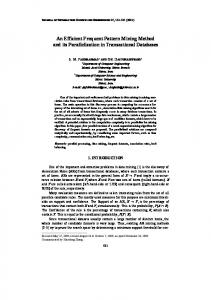
2.1 Relationship of colossal pattern to other patterns The growth process of a colossal pattern is depicted in figure 2. Let minimum support be 50. When the pattern A is extended with pattern B, then the frequency of AB drops to 198. This indicates that pattern A occurs 200 times, out of which it occurs along with B 198 times. The pattern AB is closed but not colossal. Growth of the pattern cannot be

IJCSNS International Journal of Computer Science and Network Security, VOL.10 No.1, January 2010 stopped at C, since extension of it by adding D has the same support as the original pattern. Pattern ABCD is closed but not colossal. Unless there is a significant difference in the frequency of the pattern when it is extended, the smaller pattern will not be considered for colossal pattern though it is a closed pattern. For example, when ABCDF is extended to include G in it, the frequency is reduced from 193 to 190 and we don’t consider ABCDF as a colossal pattern instead ABCDFG is a colossal pattern. When ABCDFG is extended with Q, there is a significant drop in the pattern’s frequency and hence this extension will not be considered as colossal pattern. (Marked with cross in figure.2) Hence ABCDFG is treated as a colossal pattern, but ABCDFGQ is a maximal pattern. Therefore a maximal pattern need not be a colossal pattern all the time. In figure 2, ABCDEH and ABCDFG are colossal patterns. The following points are observed, through the above example: • •

Every colossal pattern is a closed frequent itemset but every closed frequent itemset need not be a colossal pattern. A colossal pattern need not be a maximal frequent itemset all the time.

200 Frequency of

pattern

198

Patterns

C

195

D F

150

E

For any itemset α, we denote the set of transactions that support α as TIDα and referred to as support set of α. Definition 1 (Frequent itemset) For a transaction dataset TID, an itemset α is frequent if

| TIDα | | TIDα | is ≥ σ , where | TID | | TID | called the support of α in TID, written supp(α) and σ is the minimum support threshold, 0 ≤ σ ≤ 1. The important characteristics of prodigious or colossal patterns are • They are lengthy by nature • They are less in number in a given database. • They are robust .That is, even if a small number of items are removed from the pattern, the resulting pattern would have a similar support set. The larger the pattern size, the more prominent this robustness is observed.

3.2. Supporting concepts for our algorithm A colossal pattern is lengthy by nature. It possesses a number of subpatterns. There can be more than one colossal pattern in a given data set. Each colossal pattern will have a huge set of subpatterns. Consider the example quoted in figure 3. It contains a colossal pattern {1 2 3 4 5 6 7 8}. It may have 8

B

195

140

A

193 190 G

H

50 Q

Figure.2 Pattern tree growth process

3. Algorithm design and overview 3.1. Basic concepts Let I={x1, x2 … , xn} be a set of items. Any nonempty subset of ‘I ‘ is called an itemset. A transaction dataset TID is a collection of transactions, TID = {t1, t2, …, tn}, where each transaction ti consists of a set of items which are contained in I.

305

8

8

c2 2-itemsets, c3 3-itemsets, c4 4-itemsets and so on. If

we use a level wise mining strategy, we may not get the mining result in a reasonable amount of time. Hence a new agglomerative strategy is required to attain the colossal patterns in less time skipping mid sized patterns. Subpatterns belonging to a colossal pattern are expected to be present in a neighborhood. We call them as core patterns. By merging the core patterns present in a neighborhood, we will attain a colossal pattern. Among these enormous numbers of subpatterns, subpatterns of a colossal pattern may overlap with the subpatterns of another colossal pattern. For example in figure 2, the sub patterns of two colossal patterns ABCDEH and ABCDFG overlap. Therefore, in order to find the neighborhood of a lengthy pattern we have to adopt a distance measure. The following metrics are used in finding the core pattern neighborhood. Definition 2 (Core Pattern) [5] For a pattern α, an itemset β ⊆ α is said to be a τ-core pattern of α if

| TIDα | ≥ τ , 0 ≤ τ ≤ 1. | TIDβ |

where τ is called the core ratio.


306

For a pattern α, let α.corelist be the set of all its core patterns. Definition 3 (Core Descendant) [5] For two patterns β and β’, if there exits a sequence of βi , 0 ≤ i ≤ k, k≥ 1 such that β = β0 , β’ = βk and βi Є βi+1.corelist for all 0 ≤ i ≤ k , β is said to be a core descendant of β’. Definition 4 (Pattern Distance) [5] For patterns βi and βj , the pattern distance of βi and βj is defined as Dist(βi , βj) = 1 -

| TIDα | Dist(α,βi) = ------------------------------------------| TIDβ1| + | TIDβ2|- | TIDβ1 ∩ TIDβ2 | = 1−

| TIDα | ≥τ | TIDβi |

| TIDβi U TIDβj |

That is, Dist(α, βi)

___________________

1 2 /τ − 1

| TIDα | | TIDβi |

Case 1: If βi is the τ-core pattern of α then

| TIDβi ∩ TIDβj |

Note: For two patterns β1, β2 Є α.corelist, Dist(β1, β2) ≤ r(τ), where r(τ) = 1 −

| TIDβi U TIDβj | by lemma 1 we have, if βi ⊆ α then TIDβi ⊃ TIDα.

= 1 - ( τ + ε ) = 1- τ - ε ≤1-τ Where ε is a small value. Case 2: if βi is a τ-core descendant of α (a) If ∃ γ such that βi is a τ-core pattern of γ and γ in turn is a τ-core pattern of α, then we have | TIDγ | | TIDα | ≥ τ and ≥τ | TIDγ | | TIDβi |

| TIDα | | TIDα | | TIDγ | = × ≥ τ ×τ | TIDβi | | TIDγ | | TIDβi |

Figure 4: Distance between any two farthest patterns ≤ r (τ) It follows that all core patterns of a pattern α are bounded in a metric space by a ball of diameter r(τ). It is possible that the ball may contain overlapping neighborhood regions of multiple colossal patterns. . In order to recognize such core patterns from the patterns enclosed in a ball of a colossal pattern, we can make use of the following restriction stated in theorem 1. Theorem 1: Let α be a growing pattern and βi be its core descendant pattern then Dist (α, βi ) ≤ 1- τ , where 0 ≤ τ ≤ 1. Proof: The distance between any two patterns is given by definition 4 as Dist (βi , βj) = 1 -

| TIDβi ∩ TIDβj | ___________________

≥ τ2 (b) If ∃ a sequence of ‘k’ γ’s as core descendants of α and βi is their core descendant, then we can prove that | TID α | ≥ τk+1 | TID β i | Hence Dist (α, βi) = 1 - (τk+1 + ε) ≤ 1 - τk+1 ≤1-τ The proof is concluded. From the above theorems 1 and 2, we can have the following corollaries. Corollary 1: | TIDα | ≤ |TIDβ | ≤ | TIDα | τ Where α is the growing pattern in which the sub pattern β is merged. Corollary 2: For β to be frequent |TIDβ | ≥ σ Hence σ ≤ | TIDβ | ≤ | TIDα | τ Based on the above two corollaries, the frequencies of the core descendants of a colossal patterns are expected to be nearer to the frequency of the colossal pattern, thereby forming a frequency band. So the core patterns of overlapping colossal patterns sharing a

IJCSNS International Journal of Computer Science and Network Security, VOL.10 No.1, January 2010 neighborhood ball can be separated in A unidimensional clustering applied on the frequencies of the pertinent core

patterns’ results in multiple frequency bands, each suggesting the constituents of a colossal pattern.

Item-IDs 1 2 3 4 5 6 7 8 9 10 11 12 13 14 15 16 17 18 19 20 21 23 25 27 28 29 32 33 34 35 36 37 38 40 43 46 47 50 55 60 1 1 1 1 1 1 1 1 3 7 2 10 1 13 12 1 6 9 9 9 9 9 9 9 9 10 10 4 13 11 14 15 2 7 12 11 13 15 7 8

12 8 1 10 10 10 8 5 3 2 10 6 2 2 6 2 10 5 5 5 10 3 4 13 11 4 14 14 14 12 11 7 9 14 10 8 6 10 3 14 13 7 6 14 5 5 16 8 11 15 11 14 16 11 9 14 8 15

Figure:3 TID-List of example While finding the distance between the growing pattern and a candidate core pattern, we need the frequencies of the patterns formed by the union and intersection operations which may require additional database scans. This was avoided by adapting vertical format representation of the elements of the initial pool. Each pattern is represented as a TID list in vertical formatting. The proposed Merger algorithm generates the growing patterns in vertical formats so that, they can be directly included in the pool for next iteration.

3.3 Colossal Pattern Miner (CPM) Overview Consider the sample database shown in table 1.Let us use the transformed database shown in figure.3. We consider minimum support σ to be 2. By using any efficient existing frequent pattern algorithm, we were able to get the 1-itemsets associated with their frequency as well as TID lists as shown in table.1. Step-wise method: 1. 2.

3.

4.

We start with an initial pool consisting of 1 or 2itemsets (can be obtained using any frequent mining algorithm). We partition the patterns in the initial pool based on their frequencies using any standard clustering algorithm as shown in figure 4 and figure 5. We call them as frequency bands. Starting from the largest frequency band, select a seed pattern ‘α’ randomly and form its neighborhood containing τ-core patterns of the seed(based on distance), selecting from the present band and next the other bands in descending order of their size. If the frequency of the patterns selected as τ-core patterns (β) is less than 1- τ remove the pattern from its parent frequency band.

307

Table 1:1-itemsets as candidate pool

pattern 1 2 3 4 5 6 7 8 9 10 11 12 13 14 15 16 17 18 19 20 21 23 25 27 28 29 32 33 34 35 36 37 38 40 43 46 47 50 55 60

frequency 2 2 2 2 2 2 2 2 4 2 4 2 3 3 2 3 4 2 3 3 2 2 2 2 2 3 3 2 4 3 3 4 2 2 2 4 3 2 3 4

TID-List 1,9 1,9 1,9 1,9 1,9 1,9 1,9 1,9 3,10,12,16 7,10 2,4,11,12 10,13 1,11,13 13,14,15 12,15 1,2,7 6,7,8,13 12,13 8,11,16 1,4,8 10,14 10,14 10,14 8,12 5,11 3,7,11 2,9,15 10,14 6,10,11,15 2,8,14 2,6,16 6,10,11,15 2,3 10,14 5,13 5,7,9,12 5,6,14 10,14 3,5,8 4,5,15,16


308

Table.2: Neighborhood of ‘5’

pattern 1 2 3 4 5 6 7 8

frequency 2 2 2 2 2 2 2 2

TID-List 1,9 1,9 1,9 1,9 1,9 1,9 1,9 1,9

Table3: Neighborhood of ‘25’

pattern 21 23 25 33 40 50

frequency 2 2 2 2 2 2

Let the randomly drawn seed pattern be ‘5’. Now we will find out the distance between ‘α’ (5) and each β, other than α, in the initial pool. We choose the value of τ as 0.5. Substituting τ value in r (τ), we have by theorem 1, r (τ) = 2/3. We use the distance measure from Definition 4. Let β=1, then Dist (5, 1) =1- 2/2 = 0 < 2/3. Therefore 1 ∈ 5.corelist. We repeat the same for all the core patterns in initial pool. Finally we get all the core patterns within the ball of ‘5’ and store them in 5.corelist as shown in the table 2. Similarly, the corelist of pattern ‘25’ is shown in table 3.

TID-List 10,14 10,14 10,14 10,14 10,14 10,14

Figure5: Partitioning the candidate pool

Figure 4:Distribution of patterns among various frequency bands

5.

6. 7.

Repeat step 3 and 4 until all the patterns are selected or until number of neighborhoods formed are equal to desired number of colossal patterns. Now we start merging the patterns in each neighborhood in order to form one or more super patterns (colossal patterns). The set of super patterns now becomes the new initial pool and the process is repeated until we attain colossal patterns.

In our running example, the entire candidate pool can be divided into (here) three bands with cluster centers 2, 3, 4 respectively. Patterns whose frequency is near to 2 are assigned to band with cluster center 2 Patterns whose frequency is near to 3 are assigned to band with cluster center 3 and so on. This is shown in the figure.4 We start with largest frequent band (here 2). We add 5 as first element and start the merging process. The pattern merging is done one at a time checking the resultant pattern’s frequency at each stage. For e.g., {1 5} U {2} is possible since 2 is not a subset of {1 5}. The union yields ‘1 2 5’. Now we check for its frequency by taking intersection of their TID lists. (t1, t9) ∩ (t1, t9) yields (t1, t9). Hence frequency of ‘1 2 5’ is 2 and it is frequent. Now ‘1 2 5’ can be merged with another pattern of the same cluster and the same process is repeated for all the patterns in each cluster. Finally the cluster with center 2 yields a colossal pattern ‘1 2 3 4 5 6 7 8’ with frequency 2. The selection of patterns during merging process: 1. Start processing the patterns from highly frequent band. 2. Let α (here 5) be the growing pattern. Initialize it to the first pattern in the band.

IJCSNS International Journal of Computer Science and Network Security, VOL.10 No.1, January 2010 3. Repeat for all the rest of patterns indexed by i, in the band and next the other clusters in descending order of their size until α cannot be extended, the following steps: i) Check whether α can be extended by merging pattern Pi. That is make sure that the pattern Pi is not a subset of α. ii) Find the intersection of TIDlists of α and Pi a) If the size of this list representing the support of growing pattern is < σ, then undo pattern growth and proceed with step 3 afresh. b) else if the distance between Pi and extended α is more than 1- τ [by theorem 2] then record α U Pi as a frequent long pattern. c) else update α = α U Pi and note the new TID list of α . 4. Record α as a colossal pattern along with its TID list. 5. Repeat steps 3 and 4 on the lower bands, starting with α initialized to first pattern. Theorem 2: Pattern extension in accordance with their distance to the seed patterns will not miss the lengthiest pattern. Proof: The sequence in which the subpatterns are merged, while forming a colossal pattern is done based on their nearness to the growing pattern. Nearness of two patterns is measured in terms of commonly shared transactions (by definition no 4). The more transactions are common to two patterns, the more closely the patterns. When two closer patters are merged, there will not be any drastic difference in their frequency. The subpatterns are arranged according to the nearness distance to the seed pattern. If the order is not considered, a sub pattern that shares lesser number of common transactions may stop the extension of the growing pattern, once it is merged to the growing pattern. Merging is done, starting with the least distant pattern (nearest sub pattern) so that, the growth will be promising and uniformity is maintained. Thus it contributes the lengthiest pattern. Observations: 1) A colossal pattern is expected to be the resultant pattern formed by merging multiple smaller frequent patterns (sub patterns) with nearly equal support to that of the colossal pattern. 2) The neighborhood of a sub pattern βi with a radius of r (τ) recognized in the theorem 1, may include multiple clusters, each yielding a super pattern. There by we can have multiple super patterns formed by a pattern’s corelist. The above observations are essential in our algorithm design.

309

3.4. Colossal pattern mining algorithms: Algorithm 1 (Main module) Input: Initial pool IP, Core ratio τ, Maximum number of patterns to mine M. Output: Set of frequent patterns C. 1: do 2: S ←Colossal Pattern Mining (IP, M, τ); 3: CandidatePool ← S; 4: while |S| > M; 5: C ←RemoveSubsets (S); 6: return C; Figure 6: Main algorithm The global algorithm is outlined in figure 6. The initial pool is generated by applying Apriori algorithm [1] up to 1 or 2 itemset level. Lines 1 to 4 are the body of the iteration, which calls the algorithm Colossal Pattern Mining. On completion of iteration, the Main algorithm checks the frequent patterns returned by Colossal Pattern Mining. If the result set contains more than M patterns, it begins the next iteration with the generated set of super patterns as candidate pool (initial pool). The function RemoveSubsets () trims the resultant colossal patterns. The output of the main module constitutes a set of resultant colossal patterns which is the desired result. Algorithm 2 (Colossal pattern mining) Input: Initial pool IP, Core ratio τ, minimum support σ, K number of clusters, Maximum number of patterns to mine M. Output: Set of super patterns S 1: S ← Ф; T ← Ф; 2: r (τ) = 1 −

1 2 /τ − 1

;

3: Clu ← Get_Bands (IP, K); // All the bands are stored in Clu 4: CluSort (Clu); 5: for i = 1 to M, j=0 to K 6: {Draw a seed α from largest cluster in IP; 7: if |TIDα| ≥ σ then 8: {for each β Є Clu (CluSort[j]) 9: if Dist (α, β) ≤ r (τ ) 10:{record triplet in αi .CoreList 11: T ← T U {α}: 12: αi .CoreList [1] ← α;} } 13: if β.freq < (|TIDα ∩ TIDβ|) + σ {Discard β from initial pool ;} }}// for in step 2 14: for each α Є T 15: S←S U Pattern_Merger (αi .CoreList); 16: return S; Figure: 7: Colossal pattern mining algorithm

310


Step 1 in figure 7 initializes the temporary variable T and the set S, which stores super patterns. Step 2 computes the neighborhood distance. Step 3 calls an algorithm Get_Bands, which partitions the patterns in initial /candidate pool, using a standard partitioning algorithm (say, a variant of K-means). All the frequency bands are stored in Clu. In step 4, the algorithm CluSort sorts bands in descending order of their band sizes. Steps 5 to 13 are the methodology for finding corelists for the M seeds drawn from K bands, starting from the largest one. In step 13, a pattern‘s (β) frequency is assessed, to see if it can participate in any other neighborhoods too. If β is not that significant, then it is removed from the initial pool. This helps in improving the algorithm’s computing time. In step 15, each corelist is taken and the patterns in the list are merged to form super patterns upon calling the algorithm Pattern_Merger shown in figure 8. Algorithm 3 (Pattern _Merger) Input: Number of core lists Cno, minimum support σ, Set of CoreList patterns. Output: Set of super patterns colossal 1: colossal =φ; temp =φ; 2: C ← Set of core lists; 3: for i = 1 to Cno 4: { α ← first pattern in Ci 5: for j = 1 to | Ci | – 1 6: {temp ← α U Pj // Pj ∈ Ci 7: if Pj ⊆ α, discard temp & continue 8: else 9: {TIDtemp ← TIDα ∩ TID Pj; 10: if | TIDtemp| < σ 11: {undo α U Pj and continue with next} 12: else if Dist (temp, α ) > 1-τ 13: {record in freqlongpatternlist; 14: undo α U Pj and continue.} 15: else 16: { α ← temp; 17: α.freq ← temp.freq; 18: TIDα ← TIDtemp ; } }//else in step 8 }//for in step 5 19:colossal ←colossal U }//for in step 3 20: Return colossal; Figure 8: Pattern_Merger algorithm Steps 1 and 2 initialize the variables. Steps 3 to 19 cover the methodology for generating super patterns. A pattern is merged with the other pattern in a corelist, only if it is not a subset of it. This is confirmed by step 7. If the merged pattern’s frequency is less than minimum support threshold, then the merging is undone with that pattern.

If upon merging the growing pattern’s frequency drops significantly, but greater than minimum support, then the merged pattern is stored, but the merging is undone and the pattern may grow in other directions. These strategies contribute to the growth of lengthy patterns. These are shown in steps 10 to 14. If the merging is useful for pattern growth, then the original pattern is updated with the new merged pattern and its frequency and transactions are also updated to continue with the next iteration to generate a lengthier pattern. This is depicted in steps 15 to 18. Finally step 20 returns a set of lengthy patterns.

4. Evaluation metrics Our proposed colossal pattern mining algorithm gives a good approximation of the entire mining result. This adds advantage when the size of the mining result is unmanageable. We need a new metric for assessing the representativeness of the set of colossal patterns to the complete mining result. Evaluation of the algorithm is done in terms of (1) Runtime (2) Representative score (Definition no-6) Definition 5 Pattern Dissimilarity (PD) The dissimilarity of β to α be defined as the ratio of number of distinct items of β which are not represented by α to the length of β. mathematically it is represented as follows: PD (α, β) = | β - (α ∩ β)| |β| PD (α, β) lies in the range of 0 to 1 which may differ from PD (β,α) and PD (α,α) is zero. Given two collections of itemsets X and Y, Y being the complete set of patterns and X being the colossal pattern mining result, we need a metric to measure how well X approximates Y. The formal definition is given as follows: Definition 6 (Representative score) The representative score is the ability of a smaller set of colossal patterns to represent the complete mining result. If X denotes the set of colossal patterns, X={x1 , x2 , …,xm} and Y denotes the set of complete mining result, Y={ y1, y2 ,…,yn}(where m is significantly smaller than n) Then the representative score of X with respect to Y, denoted as RS(X, Y) is given as RS(X, Y) = i=1 to m ∑ RS(xi) ___________ m where RS (xi) = 1- PD(xi ,y ) + Dist(xi ,y ) 2 Procedure to find the representative ness of X to Y:

IJCSNS International Journal of Computer Science and Network Security, VOL.10 No.1, January 2010 Step-1: Taking each colossal pattern as a medoid the elements of Y are distributed into various clusters with nearest medoid (Definition no.4 is taken as distance measure.) Step-2: The farthest pattern ‘y’, from the medoid over all the elements in the cluster is identified. Step-3: The representative score of a colossal pattern is defined as follows: RSi (xi) = 1- PD(xi ,y ) + Dist(xi ,y ) 2 Step-4: The representative score of the set of colossal patterns is the average of the individual representative score of its members. Representative score lies between 0 and 1. As RS reaches 1, it shows maximum approximation of X in representing Y. The best representation set gets the score nearer to 1. Illustration For example, consider a complete set Y= { 1,2,3,4,5,6,7,8,9,10,11}. Let the colossal mining result be set X= {(7, 8, 9, 10, 11), (1, 2, 3, 6)}. Given their respective tidlists (we considered Diag 6 data for illustrating the representative scores), the representative score of X to Y are tabulated in table 4 Table.4 Representative scores of the two clusters.

Cluster 1 RS(x1, y1 ) = 1-0.15=0.85 RS(x1, y2 ) = 1-0 =1 RS(x1, y3 ) = 1-0.15=0.85 RS(x1, y4 ) = 1-0.15=0.85 Maximum over cluster 1 = 0.85 Cluster 2 RS(x1, y5 ) = 1-0=1 RS(x1, y6 ) = 1-0.25=0.75 RS(x1, y7 ) = 1-0.25=0.75

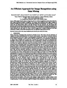
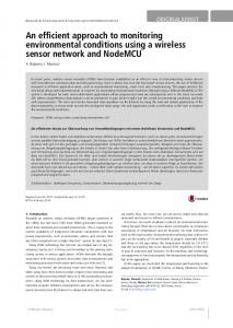
algorithm Colossal pattern Miner (CPM) against Closet+ [10]. Data characteristics: We applied CPM algorithm on Yeast data [4]. The result, from an experiment with n genes on a single chip, is a series of n expression-level ratios. Typically, the numerator of each ratio is the expression level of the gene in the varying condition of interest, whereas the denominator is the expression level of the gene in some reference condition. The data from a series of m such experiments may be represented as a gene expression matrix, in which each of the n rows consists of an melement expression vector for a single gene. The expression measurement is positive if the gene is induced (turned up) with respect to the reference state and negative if it is repressed (turned down). Experiments are carried out using a set of 79-element gene expression vectors for 2467 annotated yeast genes. The data were collected at various time points during the diauxic shift, the mitotic cell division cycle, sporulation, and temperature and reducing shocks, and is available via the Stanford web site. We considered the first 110 genes. Thus our data constitute 110 rows and 79 columns. We mined frequent patterns in yeast data. The runtime is shown in figure 9. The synthetic data Diag 40 [5] is checked for quality which is depicted in terms of representative score in figure 10. The graph depicts the comparative statement in terms of Representative Scores of the set of colossal patterns versus equal sized uniform sampling taken from all frequent itemsets. It may be observed that the set of colossal patterns represents the all frequent itemsets better than random sampling. It can also be observed that as the size of the representative set increases, the representative score also increases, which coincides with the natural expectation and hence the proposed metric supports natural intuition.

Maximum over cluster 2 = 1 RS(x, y ) = 0.9 As the RS value approaches ‘1’, it better represents the complete mining set.

311

closet +

CPM

6000

5000

4000

3000

2000

5. Results 1000

In this section, we demonstrate both the performance study of our algorithm over synthetic datasets and application on real-time dataset. All of our experiments are performed on a 2.00GHz, 1 GB memory Intel PC, running Windows XP. We implemented the algorithm in Java. We evaluated our

0 10

8

6

5

4

3

M i n i m u m su p p o r t ( %)

Figure 9: Runtime on yeast data

2


312

Conclusions We studied a technique for mining colossal patterns [5] and implemented our own strategy of mining colossal patterns. Instead of randomly picking a seed pattern, we suggest to pick up the seed pattern in an intelligent way. We suggest a way of separating sub patterns of overlapping colossal patterns based on their frequencies which facilitates leaping through the enormous number of mid sized patterns. We also suggested adopting vertical data format in order to avoid repeated database scans, while finding the distance between a pair of core descendant patterns. CPM

uniform sampling

0.9 0.8 0.7 0.6 0.5 0.4 0.3 0.2 0.1 0 50

100

150

200

300

350

400

N umb er o f mined p at t er ns

Figure 10. Representative score for Diag 40

References [1] R.Agrawal, T.Imielinski, and A. Swami. Mining association rules between sets of items in large databases. In SIGMOD’93, pp 207-216, Washington, D.C., 1993. [2] R.Agrawal, H.Mannila, R.Srikant, H.Toivonen and A.Inkeri Verkamo. Fast discovery of association rules. In ‘Advances in Knowledge Discovery and Data Mining’, pages 307-328, AAAI press, Menlo Park, CA, 1996. [3] R.J.Bayardo. Efficiently mining long patterns from databases. In ACM SIGMOD conf. Management of Data, June 1998. [4] J.Han, J.Pei and Y.Yin. Mining frequent patterns without candidate generation. In ACM SIGMOD conf. Management of Data, May 2000. [5] Zhu.F et al., Mining colossal Frequent patterns by core Pattern Fusion In: Proceedings of the 2007 international conference on Data Engineering, Istanbul, Turkey. [6] Madhavi D & M.Shashi, An Efficient Algorithm to Mine Prodigious Frequent Patterns In: Proceedings of the 2008 international conference IISA’08, UCONN, New York. [7] Survey of Clustering Data Mining Techniques-Pavel Berkhin Accrue Software, Inc. [8] J.Han and M.Kamber. Data Mining concepts and Techniques, Morgan Kaufmann publishers, SanFrancisco, CA, 2001.

[9] N.Pasquier, Y.Bastide, R.Taouil and L.Lakhal. Discovering Frequent Itemsets for association rules in ICDT 1999. [10] J.Wang, J. Han, and J. Pei. Closet+: Searching for the best strategies for mining frequent closed itemsets. In KDD’03, pages 236–245. [11] http://genome-www.stanford.edu/ D.Madhavi received her M.sc. Degree in Computer Science from P.B. Siddhartha college, Vijayawada and M.E. Degree in Computer Engineering with distinction from Andhra University. She is presently working as an Associate Professor in the department of Computer Science and Engg, Pydah College of Engineering and Technology, Visakhapatnam, Andhra Pradesh, India. She is pursuing her Ph.D from Acharya Nagarjuna University. Her areas of interest include Data Mining, Information Retrieval, and Data base systems. M.Shashi received her B.E. Degree in Electrical and Electronics and M.E. Degree in Computer Engineering with distinction from Andhra University. She received Ph.D in 1994 from Andhra University and got the best Ph.D thesis award. She is working as a professor and HOD of Computer Science and Systems Engineering at Andhra University, Andhra Pradesh, India. She received AICTE career award as young teacher in 1996. She is a co-author of the Indian Edition of text book on “Data Structures and Program Design in C” from Pearson Education Ltd. She published technical papers in National and International Journals. Her research interests include Data Mining, Artificial intelligence, Pattern Recognition and Machine Learning. She is a life member of ISTE, CSI and a fellow member of Institute of Engineers (India).