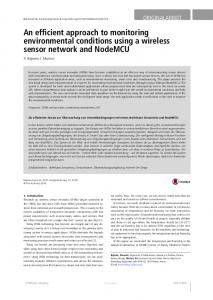
Figure 1 Circle-circle intersection. First, how the Cross-Plot captures clusters in a data set is described. Assume a perfect uniformly dense circle D of radius R.
An Efficient Approach to Detect Cluster Locations using Cross-Plots Kelvin Wong Kian Loong Sanjay Chawla
School of Information Technologies University of Sydney NSW 2006, Sydney Australia {kwon6729, chawla}@usyd.edu.au
ABSTRACT In this paper the Cross-Plot [1,3] framework is extended to efficiently detect the location of clusters. This is achieved by placing elemental nodes around the data regions and then computing their corresponding Cross-Plots with the data set. For a single elemental node and a single perfect cluster, the point of inflexion of the Cross-Plot provides a good indication where the center of the cluster lies. It turns out that this approach seems to be insensitive to outliers and noise in the data. Furthermore, the approach is scalable to arbitrarily many clusters.
Categories and Subject Descriptors
H.2.8 [Database Applications]: Data mining; H.3.1 [Content Analysis and Indexing]: Abstracting methods; H.3.7 [Digital Libraries]: Collection
General Terms Algorithms
Keywords
Spatial data mining, fractal dimension, intrinsic dimension, pair correlation, correlation integral
1. INTRODUCTION
Clustering is one of the core data mining techniques. It is extensively used as a mechanism to summarize large quantities of data into a few meaningful labels. For example, an online store can partition its customer base into a few meaningful clusters based on the web-usage information of the customers. This information can then be used to create customized product catalogs for each cluster. A good clustering tool should insensitive to noise and should internally use a “denoising” function to smooth data brittleness. The cluster analysis should still be able to support classification of attributes from the data set, even if noise is present. Permission to make digital or hard copies of all or part of this work for personal or classroom use is granted without fee provided that copies are not made or distributed for profit or commercial advantage and that copies bear this notice and the full citation on the first page. To copy otherwise, or republish, to post on servers or to redistribute to lists, requires prior specific permission and/or a fee. Conference ’00, Month 1-2, 2000, City, State. Copyright 2000 ACM 1-58113-000-0/00/0000…$5.00.
Clustering is an extremely well researched topic and various methods exist in literature. Of late, new generation methods based on fractal analysis have emerged. One such method is based on the notion of Cross-Plots, which uses the notion of relative distance to obtain global summary information about the data sets. Cross-Plots have been used to answer important questions about the relationship between two data sets [3]. For example, (1) Do the data sets come from the same distribution? (2) Do they repel each other? (3) Are they close or far away? (4) Are the data sets separable and finally (5) Given an unlabelled point, which of the two sets does it come from (if any). The concept of Cross-Plot is used to answer the fundamental question in clustering analysis. Given a single non-uniformly distributed data set determine the center of its clusters. It turns out that by placing a few artificial nodes (or elemental nodes) around the data set and creating Cross-Plots between these nodes and the data set, the cluster centers can be determined in an extremely efficient manner. In fact because this method is extremely efficient it can also track moving clusters in near real-time. The rest of the paper is organized as follows. In section 2 existing work has been briefly surveyed in the data mining community vis-à-vis tracking of moving clusters. In Section 3 the overview of the technique known as GeoPlot was briefly described as it is central to approach. Our proposed approach of cluster tracking using concepts from the GeoPlot is formulated in section 4. Section 5 discusses the performance of the tracking technique and its limitations. Finally, the last section concludes the paper and provides possible future developments.
2. RELATED WORK
The interest in mining useful information from the massive wealth of knowledge in the world has resulted in various data mining tools developed over the past decade. J. Y. Pan and C. Faloutsos suggested the use of GeoPlot to analyze patterns on spatial data information. In their approach, GeoPlots of datasets are computed, which revealed important data characteristic information. The intrinsic (fractal) dimension is a good representation of real world data [2,3], where characteristics at both local and global scales can be considered at the same time. Hence GeoPlot is able to discover correlations among spatial objects at both local and global scales [1].
3. BACKGROUND
This section discusses the theory of Cross-Plot [2][6] and how it can be used for capturing the distributional properties of a multi-dimensional data set. It is particularly interesting to know how clusters in a data set are manifested in these plots.
3.1 Mathematical Formulation of Cross-Plot
First, how the Cross-Plot captures clusters in a data set is described. Assume a perfect uniformly dense circle D of radius R centered at a distance d from an elemental node p as shown in Figure 1. For a circle of varying radius r centered at p, the number of points N(p,D,r) which are in the intersection of the two circles is proportional to the area of the circle-to-circle intersection. In particular this area Area(p,r,D) is given by [7]:
d 2 � R2 � r 2 )� 2dR
A Cross-Plot is defined as a plot of the logarithm of the number of counts of object pairs that do not exceed a specified proximity distance versus the logarithm of this varying proximity distance. More formally:
r 2 cos 1 (
Definition 1. Cross-Plot between two data sets A (with NA points) and B (with NB points):
1 ((�d � R � r )(d � R � r )(d � R � r )(d � R � r )) 2 2
Area( p, r , D)
R 2 cos 1 (
d 2 � r 2 � R2 )� 2dr
1
§ N �r · Cross A, B �r log¨¨ A, B ¸¸ © NA NB ¹
versus log�r
where NA,B(R) is count of object pairs within distance r. Definition 2. points):
Thus N(p,D,r) =� $UHD(p,r,D) where is the density of the circle. Based on the above equation, If two uniformly dense circle D1 and D2 of radius R1 and R2 centered at (d1,0) and (d2,0) respectively, and an elemental node p located at the origin as shown in Figure 2 (a). The CrossD, (r) can be computed as shown in Figure 2 (b).
Self-Plot of a given data set A (with NA �
Self A �r log �
�
�
�
N A, A �r N A � N A 1 2 �
versus log�r
�
�
�
�
�
where NA,A(R) is count of object pairs of set A within distance r. Definition 3. The GeoPlot of two data sets A and B is the graph which consists of Cross-Plot of A and B, CrossA,B(R), and the Self-Plots of both data sets, SelfA(R) and SelfB(R).
3.2 Cross-Plot of Data Set with a Single Node
Figure 2(a): Location of node and perfect circles
Cross-Plots are generally used to identify interesting patterns (clusters, for example) in complex data sets. Since the notion of Cross-Plot is defined in terms of relative distance between two types of point sets they do not provide information about the location of these patterns. The objective is to extract the location information about clusters by judiciously placing nodes around the data set and computing the Cross-Plots with respect to these nodes.
Figure 2(b): Cross-Plot of Node-Perfect Circles
Figure 1 Circle-circle intersection
The curve clearly shows that the Cross-Plot captures the sweep through the cluster (or circle) in the region just before the plateau. The plateau region is the location where no new data points are accumulated until the expanding radius reaches the next cluster. In fact the growth in the accumulation of points de-accelerates just after the midpoint of the circle. This is the inflexion point where the second derivative of Area(p,r,D) changes signs from positive to negative. Let r0 be the inflexion point of Area(p,r,D). The key observations in this paper are:
(1) The center of the cluster lies close to the boundary of a circle of radius r0 centered at p. (2) The center of the cluster can be approximated by using the point of inflexion of another Cross-Plot centered at another elemental node. This is achieved as follows. Plot two circles centered at the elemental nodes of radius equal to their length of the point of inflexion (in the anti-log space). The actual cluster center can be derived from the intersection information of these two circles. (3)
Even in the presence of limited “noise” the center of the cluster remains close to the point of inflexion of the Cross-Plot. This is because the log term in the CrossPlot has a “denoising” effect.
(4) When several clusters are present then the placement of elemental nodes can (in many instances) be derived from the global properties of the data set.
3.3 Observations of Cross-Plots
Some important observations of Cross-Plots relative to the position of elemental nodes are summarized below: Observation 1.
Analysis of pattern characteristics
The flat portion or plateau of the curve in the Cross-Plot with data set and node p indicates the existence of clusters in the data set. The number of plateaus corresponds to the number of clusters. This can be illustrated in Figure 3 below:
(a) Cross-plot with three (b) Clusters-distribution of plateaus corresponding to pattern and positioning of the three-cluster data set elemental node Figure 3: Cross-Plot (a) of 3-clusters data set with a single node as shown in (b) Observation 2.
(a) Boundary values obtained (b) Boundary encapsulation of from the Cross-Plot cluster after anti-log Figure 4: Encapsulating cluster occupation using Cross-Plot of data set and single node Observation 3.
Monitoring pattern of different orientation
Different positioning of the tracking node produces different Cross-Plot curvature during monitoring of the pattern. Figure 5 (a) shows the corresponding Cross-Plot of the pattern and node when the node is placed at equal distance from two clusters (Figure 5 (b)). The number of plateaus is the same as if there had been one cluster. But two plateaus can be observed in their CrossPlots (Figure 6 (a)) if the node is positioned along the axis or plane joining two clusters as shown in Figure 6 (b).
(a) Single-plateau Cross-Plot (b) Single boundary tracking with one point of inflexion using one inflexion point Figure 5: Orientation 1: Node positioned at equal distance from the two clusters
Extraction of pattern information
To locate the clusters in a data set, first, the values of the distance bounded by the plateau should be extracted. Note that these values are in the logarithm scale; so converting them by exponentiation allows the actual distance in metric scale to be obtained. The clusters are found to lie in the radial distance extended from the node. Figure 4 shows how to map the values from the Cross-Plot graph back to radial distance in the real world coordinates.
(a) Double-plateau boundary (b) Double boundary tracking with two points of inflexion using two inflexion points Figure 6: Orientation 2: Node positioned at different distance from the two clusters
Observation 4.
Tracking clusters
It was realized that using, the logarithmic distances at the start of the plateaus of the Cross-Plot curve and converting them into radial distances extended by the node always maps the boundary to the inside of the clusters. These values are shown to be statistically adequate to track the position of a pattern with any number of clusters. This claim was demonstrated by mapping the logarithmic distances at the start of the single- and double-plateau reflected in the Cross-Plots of a two-cluster pattern with a node into spatial distance extended from the node. Figure 5 (a) and 6 (a) show the extraction of the logarithmic distances and Figure 5 (b) and 6 (b) show the tracking of clusters based on these distances.
4. PROPOSED METHODS
This section describes the proposed approach to locate the center of clusters by using a family of Cross-Plots. Each CrossPlot is computed by placing elemental nodes that are derived from global information about the data set. In particular, information about the center of gravity of the data set can be often used to place the elemental nodes. Two methods were proposed to locate the center of the clusters. The first method is restricted to two clusters but is very accurate and efficient, in that it can detect the exact location of the cluster centroids from the Cross-Plots. The second method applies to arbitrarily many clusters and partitions the data space into curvilinear regions where the clusters reside. This method is less accurate compared with first one but is extremely efficient.
cluster locations as shown in Figure 7 (a). But when the CrossPlot produces two plateaus, then double-boundaries interception for each cluster center needs to be carried out (Figure 7 (b)). The two averages of the interception pairs for each of the two sets of boundaries are the prediction for the centers of the clusters.
(a) Orientation 1: (b) Orientation 2: Nodes perpendicularly distanced Nodes positioned along the from orientation of pattern axis of orientation of pattern Figure 7: Different orientations for tracking nodal positions Based on the understanding of the theory and observations of the Cross-Plots of pattern and nodes discussed in the previous sections, the pseudo code of our method is formulated: 1)
Compute the center of gravity or centroid, c of the global pattern D.
2)
Compute two points and such that the imaginary line joining them or the extension of this line passes through c. i.e. calculate a vector from the c to any data point in D and place one of the elemental nodes on an axis orthogonal to this vector and passing through the centroid. The other node can be places directly on c.
3)
Obtain CrossD, and CrossD, �
4)
Determine the inflexion point(s) of the two Cross-Plots. Compute their anti-log values.
5)
Form two circles centered at the elemental nodes of radius equal to their anti-log inflexion values.
6)
Derive the interception coordinates analytically. These are the approximation of the cluster centers.
4.1 Boundary Intersection Approach
To simplify the analysis, assume the presence of two local mobile clusters in a globally static pattern. In this approach, only two mobile nodes will be sufficient to track the location of the moving clusters. This approach is based on the concept of determining the starting and ending values of the plateau and remapping them as radial boundaries onto the pattern. It is illustrated previously in Observation 4 and is simple and fast to implement. Two scenarios need to be considered during the implementation of the tracking algorithm. In the first one, the positions of the nodes may evolve along an axis or plane that is perpendicular to an imaginary line joining the centers of the two clusters. Based on orientation 1 in Figure 7 (a), the prediction of the center of the clusters by intercepting the radial boundaries of the two nodes was attempted. The second scenario occurs when the nodes evolve to a position that lies along the axis of the imaginary line joining the two clusters. Four boundaries values will be obtained from the CrossPlot in this case. The tracking requires more computation as this time the interception of the start boundaries of the first plateau for node 1 and 2 gives the first cluster location, and that of the second plateau gives the second cluster location. This can be illustrated in Figure 7 (b). To improve the tracking algorithm, a case-by-case basis for tracking needs to be considered. If only one plateau is present, then the interception of the two boundaries will produce two
Figure 8 shows results of the above procedure applied to a simple two-cluster data set. To illustrate the effect of log as a “ denoising” function, noise has been added to the data set. Each frame in the Figure corresponds to a different time-step. In effect the clusters are moving. This approach can accurately detect the cluster centers at each time-step. In particular even when the clusters collide, the method is still able to detect the cluster centers. Because of the efficiency of the algorithm O(N) where N is the number of data points, our method can be used for efficiently tracking clusters in real time. Limitations of Boundary Intersection Approach: (1)
This approach is limited to two clusters.
(2)
It is difficult to detect the orthogonal vector to place the elemental nodes. However in practice the only restriction is that the line joining the two elemental nodes should pass through the center of gravity of the data set D.
Time frame 1
Time frame 2
6)
The mapped values are portrayed as boundary of radius ri,j extended from the center of the nodes such that i represents the node symbol and j represents the number of boundaries,
7)
For nodal positions given by (ix, iy), the regions occupied by the pattern, R(x, y) is partitioned into labels, Pi,j such that
where ri,1 < ri,2 …< ri,m-1 ,
Assign
Time frame 3
Time frame 4
R(x, y)
i
{ �� }
�Pi,j ,
if
(ri,j) ����x - ix) 2 + (y - iy) 2 ) < (ri,j+1),
where
Pi,j
�
{1 .. n n }, i
{ �� }.
8)
Label the point (x,y) in the data set according to the partition region that it falls into. i.e. Dlabel(x, y) = R(x, y).
9)
Compute the center of gravity for all the data points with the same label.
Limitations of the Technique
Time frame 5
(1)
When more than one clusters overlap during projection onto a plane, the detection of plateaus fails and the boundaries cannot be created. This occurs when the clusters are very close to each other. The problem generates failure of cluster detection for both two and more than two clusters pattern.
(2)
There has not been an ideal algorithm for detecting plateaus in the Cross-Plots of the pattern and elemental nodes as yet. The technique of histogram plotting and selection of the largest count as the plateau of the Plot is merely an estimation of the location of the plateaus, and is described in the next section.
Time frame 6
Time frame 1
Time frame 2
Time frame 3
Time frame 4
Time frame 5
Time frame 6
Figure 8: Tracking of clusters using 2 mobile nodes with the line joining them passing through center of gravity of pattern
4.2 Region Partitioning Approach
In order to lift the limitations of the Boundary Intersection approach we now propose another algorithm which partitions the data regions based on the Cross-Plots. The algorithm (described below) partitions the data space using information about the midpoint of the plateaus in the Cross-Plot. The mid-point of the plateaus correspond to the separation between clusters. 1) 2)
Calculate the center of gravity or centroid, c of the global pattern D.
Place two elemental nodes, D= ( x� y)� and E=( x, y), one on each of the two orthogonal axes that are radiated from the point c. The nodes should be on the frame which encloses the data set D.
3)
Compute the Cross-Plots, CrossD, and CrossD, �
4)
From each of the two Cross-Plots, identify the mid-points of all the plateaus, excluding the one with the largest log(countof-pairs) value. (i.e. The last plateau on the right of the curve)
5)
If there are n and n such mid points corresponding to each of the two nodes, map the log(r) values that correspond to the mid-point of the plateaus into real space coordinates by performing exponentiation on the values (through an anti-log function).
Figure 9: Partitioning of three clusters using 2 mobile nodes lying on orthogonal axes from the center of gravity of data set
4.3
Detection of Plateaus in Cross-Plot
The following algorithm serves as the engine for detection of plateaus appearing in the Cross-Plot and helps to establish location of the clusters (by using the points of inflexion of plateaus for two-cluster tracking and the mid-points of plateaus for detecting n-cluster locations).
the the the the
1)
Quantize of the log of count pairs values into bins of size sk, such that the value of the bin is denoted by yk, where k is the number of bins.
2)
Obtain the histogram of the number of items in yk versus the bin values for all values of k.
3)
Bins with approximately the same number of items are merged together and a new bin value is allocated.
4)
The bins with the number of items that exceed a certain threshold, t are assumed to be the y-coordinates of the plateaus (i.e. log(count-of-pairs) values).
5)
An additional check is carried out such that neighboring bins have number of items sufficiently lower than the selected bins.
6)
For every bin values, the x-coordinates of the bin values are retrieved from the Cross-Plot. This is the set of the logarithmic boundary values, log(r) that falls within the plateaus.
7)
The first item of the logarithmic boundary set is approximated to be the point of inflexion of the CrossPlot. The average of the first and last item in the set is approximated to be the partition boundary.
6. CONCLUSION
In this paper the Cross-Plot framework has been extended to detect cluster centers for arbitrarily distributed clusters. Two new methods were proposed. The first method is based on extracting the point of inflexion of the Cross-Plot and leads to very accurate determination of the cluster centers. The second approach is based on determining the plateau mid-points from the Cross-Plot and used to partition the data space into regions where the clusters lay. Both methods require the placement of “ elemental nodes” which are used to create Cross-Plots. For the method to work, it is important that plateaus corresponding to clusters appear in the Cross-Plot. This can be achieved by mapping the data space into topologically equivalent one such that the separation between clusters increases. For multi-dimensional data clustering, the understanding and harnessing of Tri-Plots is recommended. Many cluster analysis using the heuristic approach suffer from the dimensionality curse and reduce cluster analysis efficiency considerably. As Tri-Plots do not suffer from this aspect [5], it is believed that the implementation of a fast computational algorithm for tracking a two-dimensional cluster-pair pattern can be extrapolated to a multi-dimensional one and with the capability to cluster patterns of higher complexity.
7. REFERENCES
[1] J. Y. Pan and C. Faloutsos. “ GeoPlot” : Spatial Data Mining on Video Libraries. Proceedings of the Eleventh International Conference on Information and Knowledge Management (CIKM'02), Mclean, Virginia, 2002.
[2] M. Faloutsos, P. Faloutsos, and C. Faloutsos. On power-law
5. DISCUSSION
The proposed approach requires only a single pass on the data set and all the information about the data set can be derived from the Cross-Plot. The strength of this technique is the element of speed. Computation is fast and the algorithm can be executed in real-time. The computation of the Cross-Plot between the pattern and the node is of complexity O(n) where n is the number of data points. Because the detection of the cluster centers can be achieved at fast speed, this technique is possible for the tracking of clusters in real time. The limitation of the region partition approach becomes apparent when several clusters are very close to each other. This is because of the difficulty in detecting the plateaus in the Cross-Plot as several clusters contribute simultaneously to the count of the node-data point pairs. This prevents plateau formation. One solution that may alleviate this problem is to map the data region into a topologically equivalent space where the separation between clusters is sufficient to form plateaus for CrossD,p(r) where p is an elemental node. Although the method for detection of the plateaus is primitive and lacks a proper analytical procedure, it is sufficient enough to predict the location of the plateaus to a certain extent that can be utilized to track clusters or partition the data region.
relationships of the internet topology. Proc. of SIGCOMM, 1999.
[3] C. T. Jr., A. Traina, L. Wu, and C. Faloutsos. Fast feature selection using the fractal dimension. XV Brazilian Symposium on Databases (SBBD), 2000.
[4] J. Roddick and Brian G. Lees. Paradigms for spatial and
spatio-temporal data mining. In Geographic Data Mining and Knowledge Discovery. H. Miller and J. Han (Eds), Taylor & Francis, 2001.
[5] A. J. M. Traina, C. Traina, Jr., S. Papadimitriou, C.
Faloutsos. Tri-Plots: Scalable Tools for Multidimensional Data Mining. 7th ACM Intl. Conference on Knowledge Discovery and Data Mining (KDD´01), San Francisco, USA.
[6] A. O. Oncel, and T. H. Wilson., Space-Time Correlations of
Seismotectonics Parameters: Examples for Japan and from Turkey Preceding the Izmit Earthquake. Bulletin of the Seismological Society of America, 92, 1, pp. 339-349, 2002.
[7] E. W. Weisstein, Wolfram Research: Eric Weisstein’s World
of Mathematics, Circle-CircleIntersection, CRC Press LLC, 1999-2003. Wolfram Research, Inc. Web Site Address: http://mathworld.wolfram.com/Circle-CircleIntersection.html