In this paper, we propose an edge preserving technique based on inverse gradient weights ... than several advanced edge preserving interpolation algorithms.
3rd INTERNATIONAL CONFERENCE ON INFORMATICS, ELECTRONICS & VISION 2014
An Efficient Edge Preserving Image Interpolation Algorithm Abhinash Kumar Jha∗ , Ayush Kumar∗ , Gerald Schaefer† and Md. Atiqur Rahman Ahad‡ ∗
†
The LNM Institute of Information Technology, Jaipur, India Department of Computer Science, Loughborough University, U.K. ‡ University of Dhaka, Dhaka, Bangladesh
Abstract—Quality degradation and computational complexity are the major challenges for image interpolation algorithms. Advanced interpolation techniques achieve to preserve fine image details but typically suffer from lower computational efficiency, while simpler interpolation techniques lead to lower quality images. In this paper, we propose an edge preserving technique based on inverse gradient weights as well as pixel locations for interpolation. Experimental results confirm that the proposed algorithm exhibits better image quality compared to conventional algorithms. At the same time, our approach is shown to be faster than several advanced edge preserving interpolation algorithms.
I. I NTRODUCTION Interpolation techniques comprise approaches designed to construct new data points from known data samples. In the case of image interpolation, data samples clearly correspond to image pixels, while interpolation is primarily employed for resampling, i.e. increasing or decreasing the image resolution. In the case of upsampling, the aim is thus to increase the per pixel density of an image and can be simply understood as the process of enlarging an image of low resolution to a high resolution version of the image. A good interpolation technique should not only preserve fine image details such as edges, but should also be computationally efficient. The following criteria should be kept in the mind when judging an interpolation technique [1]: • • • • • • • •
Geometric invariance: preserving the geometry and relative sizes of objects in the image; Contrast invariance: maintaining the luminance of objects and the overall contrast of the image; Noise: no noise or artefacts should be introduced; Edge preservation: preserving edges and boundaries, sharpening them where possible; Aliasing: no zagged or staircase edges should be introduced; Texture preservation: textured regions should not be blurred; Oversmoothing: no undesirable piecewise constant or blocky regions should be introduced; Application awareness: the produced results should be appropriate for the type of image and order of resolution (for example, they should appear realistic for photographic images, but typically require crisp edges and high contrast for medical images; if the interpolation is for general
• •
images, the method should be independent of the type of image); Sensitivity to parameters: should not be too sensitive to internal parameters that may vary from image to image; Computational efficiency: should not be computationally inefficient.
A variety of interpolation techniques have been introduced in the literature. Nearest neighbour interpolation [2], billinear interpolation [3], bibcubic interpolation [4] and spline interpolation [5] are some of the most well known and widely used algorithms for this purpose. Nearest neighbour interpolation involves the translation of known pixel values, while in billinear interpolation the average value of the nearest pixels on either side is used. Bicubic interpolation involves the translation of a weighted average of the nearest pixels, whereas spline interpolation involves a special type of piecewise polynomial as the interpolant. Unfortunately, while being of low computational complexity, these approaches suffer from insufficient preservation of spatial details in the image and consequently lower image quality. In contrast, interpolation algorithms that aim to preserve edge structures are computationally more complex. Li and Orchard [6] proposed the edge directed interpolation algorithm (NEDI), in which missing pixels are interpolated based on the estimated covariance of the high resolution (HR) image from the covariance of the low resolution (LR) image. Ketan and Oscar [7] employed an autoregressive method using GaussSeidel optimisation that relies on both LR and HR pixels. Jaiswal and Jakhetiya [8] presented an algorithm based on downsampling and using least squares estimation. Jaiswal and Kumar’s algorithm [9] is less complex and based on a set of predictors; however these predictors do not adapt well to all types of images. Oscar and Chan [10] suggested a content adaptive interpolation scheme which is computationally simple but fails to give sufficiently high image quality. In this paper, we propose an image interpolation algorithm that is not only capable of preserving edges and leading to good image quality but is also computationally efficient. II. P ROPOSED ALGORITHM The pixels of the image I are classified into four categories based on their spatial locations: odd-odd, odd-even, even-odd and even-even as laid out in Fig. 1.
978-1-4799-5180-2/14/$31.00 ©2014 IEEE
3rd INTERNATIONAL CONFERENCE ON INFORMATICS, ELECTRONICS & VISION 2014
where the weight W is the inverse gradient weight and is computed as ⎧ D ⎪ 0.5 if dD 1 = d2 =0 ⎪ ⎨ dD D ]−1 if dD W = [1 + d1D . (3) 1 > d2 2 ⎪ D ⎪ ⎩[1 + d2 ]−1 if dD ≤ dD 1
dD 1
Fig. 1.
Sign convention used in the paper.
The initial stage of the algorithm consists of filling the oddodd locations of the HR image I which are directly translated from the LR image S as I2i−1,2j−1 = M (Si,j ),
(1)
which is illustrated in Fig. 2. The remaining pixels are filled in the following two stages.
2
As can be seen, the distribution of weights is defined so that equal weights (0.5) are assigned to spatial locations where no edges can be found and the majority of weights falls in the region which dominates the edges the most, resulting in preservation of edges. B. Prediction using LC Prediction of the remaning pixels (odd-even and even-odd) is performed based on a weighted sum of neighbouring pixels as I(i,j)
=
WN (Ii,j−1 + Ii,j+1 ) + (4) WF ((Ii−2,j−1 + Ii−2,j+1 + Ii+2,j−1 + Ii+2,j+1 ),
where weights WN and WF are based on LC and calculated as 1 1 WN = (5) 2 1 + P2 and WF =
1 P1 21+
2 P
.
(6)
Here, P is a position factor, which is found to be different (and hence can be optimised) for different kinds of images. Fig. 4 shows the two weights as a function of P . Fig. 2.
Translation of odd-odd pixels from LR to HR image.
A. Prediction using inverse gradient weights In this stage, prediction of pixels is performed so that the fine detailed information of the nearest 4 neighbours of the current spatial location LC is included. Suppose (dS1 , dS2 ) and D (dD 1 , d2 ) are the sum and difference respectively of the current diagonally opposite neighbouring pixels of LC (i, j) as shown in Fig 3.
Fig. 4.
Plot of WN and WF vs. P .
Through extensive experiments, it can be concluded that the majority of edges – and hence image quality – depends predominantly on these weights. Fig. 3.
Diagonal pixels taken in pair marked with the same colour.
Then, the filling of even-even locations is goverened by 1 (2) I2i,2j = [W dS1 + (1 − W )dS2 ], 2
III. E XPERIMENTAL RESULTS To measure both efficacy and efficiency of our algorithm, we carried out an extensive set of experiments. All calculations were carried out on system with an Intel CoreT M i3-3130M Processor (3M Cache) 2.6GHz processor. A grayscale image
978-1-4799-5180-2/14/$31.00 ©2014 IEEE
3rd INTERNATIONAL CONFERENCE ON INFORMATICS, ELECTRONICS & VISION 2014
TABLE I PSNR COMPARISON OF DIFFERENT INTERPOLATION TECHNIQUES ON THE IMAGES OF F IG . 5.
Fig. 5.
The 10 test images used in the experiments.
database [11] comprising a total of 10 images, all of resolution 512 × 512, were used for the experiments as shown in Fig. 5. In order to put our obtained results into context, we have implemented five other interpolation techniques: bilinear interpolation [3], bicubic interpolation [4], content adaptive interpolation (CAI) [10], context-based image dependent (CBID) interpolation [9], and context-based image independent (CBII) interpolation [9]. A visual comparision demonstrating edge preservation quality is given in Fig. 6, which shows an original image together with interpolated versions obtained by all tested methods followed by edge detection using a Canny edge detector. It can be confirmed that our proposed approach is capable of correctly preserving more edges when compared to the other techniques. A visual comparison of resulting image quality can be found in Fig. 7, which shows a sample image interpolated using the
image 1 2 3 4 5 6 7 8 9 10 average
bilinear 29.34 22.57 25.91 32.00 32.49 29.45 26.94 28.48 27.92 26.53 28.16
bicubic 29.22 22.49 25.81 31.98 32.43 29.40 26.75 28.49 27.73 26.41 28.07
CAI 30.87 24.11 27.20 34.82 33.82 31.14 28.67 31.62 30.29 28.13 30.07
CBID 30.92 24.49 27.96 34.50 33.90 31.06 28.00 31.54 30.23 28.12 30.07
CBII 30.89 24.37 27.85 34.57 33.89 30.97 28.78 31.32 30.17 28.01 30.08
proposed 31.33 24.92 28.41 34.96 34.35 31.51 29.20 32.15 30.67 28.20 30.57
different techniques. Again, it is apparent, that our proposed algorithm yields high image quality in comparison with other methods. To obtain an objective measure of image quality, we employ the standard peak signal-to-noise ratio (PSNR) defined as PSNR(O, I) = 10 log10
2552 , MSE(O, I)
(7)
where MSE(O, I) is the mean squared error between the original image O and I is the interpolated image I generated from the downsampled version S. At the same time, we measure the running times of the various algorithms. PSNR results for all images in the dataset are given in Table I, while timing results are listed in Table II. As can be seen from Table I, our algorithm works well in comparison to the other methods we implemented. In fact, over the 10 images, it is shown to give the highest PSNR. At the same time, while not quite matching the efficiency of bilinear or bicubic interpolation, it vastly outperforms the more complex techniques in terms of computational complexity. Thus, our approach is shown to provide a fast interpolation algorithm that is capable of achieving high image quality due to its edge preserving behaviour. IV. C ONCLUSIONS In this paper, we have presented a computationally efficient edge preserving interpolation algorithm. Our proposed approach interpolates the image by prediction using inverse gradient weights as well as weights found experimently based on the current location within the image. A relationship between TABLE II RUNTIME COMPARISON [ MS ] OF DIFFERENT INTERPOLATION TECHNIQUES ON THE IMAGES OF F IG . 5.
Fig. 6. Example demonstrating egde preservation of different interpolation methods.
image 1 2 3 4 5 6 7 8 9 10 average
bilinear 80.52 76.01 78.64 89.32 83.87 86.12 74.91 84.13 82.40 75.93 81.19
978-1-4799-5180-2/14/$31.00 ©2014 IEEE
bicubic 88.75 77.96 84.27 80.93 86.73 87.96 87.35 83.88 83.03 86.17 84.70
CAI 804.34 788.33 758.86 750.39 766.56 716.35 729.08 751.64 723.48 748.23 753.73
CBID 531.11 640.08 527.89 503.98 507.80 509.73 535.11 522.25 496.44 513.42 528.78
CBII 1022.30 1013.37 898.25 892.16 929.98 930.21 920.03 939.81 918.74 952.16 941.70
proposed 190.69 209.47 198.84 193.80 202.17 220.24 199.92 177.33 205.53 216.43 201.44
3rd INTERNATIONAL CONFERENCE ON INFORMATICS, ELECTRONICS & VISION 2014
original
bilinear
bicubic
CIA
CBID
CBII
proposed
Fig. 7.
Comparison of sample image interpolated by different interpolation methods.
the predicted pixel and its surrounding is confirmed, and our algorithm if found to yield not only improved image quality since preserving fine edges but also to be computationally more efficient compared to other, more complex, methods. R EFERENCES
[9] S. Prasad Jaiswal, V. Jakhetiya, A. Kumar, and A. K. Tiwari, “A low complex context adaptive image interpolation algorithm for realtime applications,” in Instrumentation and Measurement Technology Conference (I2MTC), 2012 IEEE International. IEEE, 2012, pp. 969– 972. [10] T.-W. Chan, O. C. Au, T.-S. Chong, and W.-S. Chau, “A novel contentadaptive interpolation,” in Circuits and Systems, 2005. ISCAS 2005. IEEE International Symposium on. IEEE, 2005, pp. 6260–6263. [11] Decsai.ugr.es., “Dataset of standard 512x512 grayscale test images,” http://decsai.ugr.es/cvg/CG/base.htm.
[1] T. Wittman, “Mathematical techniques for image interpolation,” Report Submitted for Completion of Mathematics Department Oral Exam, Department of Mathematics, University of Minnesota, USA, 2005. [2] R. Franke, “Scattered data interpolation: Tests of some methods,” Mathematics of computation, vol. 38, no. 157, pp. 181–200, 1982. [3] J. Allebach and P. W. Wong, “Edge-directed interpolation,” in Image Processing, 1996. Proceedings., International Conference on, vol. 3. IEEE, 1996, pp. 707–710. [4] F. N. Fritsch and R. E. Carlson, “Monotone piecewise cubic interpolation,” SIAM Journal on Numerical Analysis, vol. 17, no. 2, pp. 238–246, 1980. [5] H. S. Hou and H. Andrews, “Cubic splines for image interpolation and digital filtering,” Acoustics, Speech and Signal Processing, IEEE Transactions on, vol. 26, no. 6, pp. 508–517, 1978. [6] X. Li and M. T. Orchard, “New edge-directed interpolation,” Image Processing, IEEE Transactions on, vol. 10, no. 10, pp. 1521–1527, 2001. [7] K. Tang, O. C. Au, L. Fang, Z. Yu, and Y. Guo, “Image interpolation using autoregressive model and gauss-seidel optimization,” in Image and Graphics (ICIG), 2011 Sixth International Conference on. IEEE, 2011, pp. 66–69. [8] S. P. Jaiswal, V. Jakhetiya, and A. K. Tiwari, “An efficient image interpolation algorithm based upon the switching and self learned characteristics for natural images,” in Circuits and Systems (ISCAS), 2011 IEEE International Symposium on. IEEE, 2011, pp. 861–864.
978-1-4799-5180-2/14/$31.00 ©2014 IEEE