AN EFFICIENT HYBRID MACHINE LEARNING METHOD FOR TIME SERIES STOCK MARKET FORECASTING O.M. Ebadati E.∗, M. Mortazavi T.†
Abstract: Time series forecasting, such as stock price prediction, is one of the most important complications in the financial area as data is unsteady and has noisy variables, which are affected by many factors. This study applies a hybrid method of Genetic Algorithm (GA) and Artificial Neural Network (ANN) technique to develop a method for predicting stock price and time series. In the GA method, the output values are further fed to a developed ANN algorithm to fix errors on exact point. The analysis suggests that the GA and ANN can increase the accuracy in fewer iterations. The analysis is conducted on the 200-day main index, as well as on five companies listed on the NASDAQ. By applying the proposed method to the Apple stocks dataset, based on a hybrid model of GA and Back Propagation (BP) algorithms, the proposed method reaches to 99.99 % improvement in SSE and 90.66 % in time improvement, in comparison to traditional methods. These results show the performances and the speed and the accuracy of the proposed approach.
Key words: time series forecasting, stock price prediction, genetic algorithm, back propagation, neural network, machine learning Received: November 11, 2015 Revised and accepted: February 13, 2018
1.
DOI: 10.14311/NNW.2018.28.003
Introduction
With the advent of the digital computer, stock market prediction has moved into the technological scope; with the growing of information technology and artificial intelligence (AI) and also the influence of financial time series, forecasting is one of the most challenging applications. Forecasting is the process of making predictions for the future, based on the past and existing data. Stock price prediction is a method by which the stock market data at a specific time in the past is processed to forecast the stock price in a future term. With the help of technology and ∗ Omid Mahdi Ebadati E. – Corresponding author; Somayeh Street, Between Qarani and Vila, Department of Mathematics and Computer Science, Kharazmi University, Tehran, Iran, E-mail:
[email protected],
[email protected] † Mohammad Mortazavi T.; Somayeh Street, Between Qarani and Vila, Department of Knowledge Engineering and Decision Science, Kharazmi University, Tehran, Iran, E-mail: mortazavie@ outlook.com
c
CTU FTS 2018
41
Neural Network World 1/2018, 41–55
intelligence models like neural networks (NNs), the time series can be predicted. In the proposed method based on date an attempt has been made to obtain a global pattern for forecasting prediction. The inputs and outputs are normalized in the [0,1] range. The resulting weights of ANN minimize the SSE without any pre-defined indicator. At first, the GA approach optimizes the weights with the SSE cost function such that desired values are calculated from a sigmoidal function. In continuation, ANN control the answers, and GA outputs decrease the iterations of ANN. Sudden changes in price of stock cause deficient accuracy when method use ANN+BP approaches together. In the beginning the GA is used for initializing the weights, and in this mechanism at the end, proposed method can work with any price of stock market (like Apple, Pepsi, IBM and etc.). Previous researches on stock price forecasting are grouped under two categories: statistical and artificial intelligence models [22]. Data of stock markets contain very useful information, and for good forecasting accuracy, a large amount of information should be considered. Stock indices usually contain four factors, which include Open, High, Low, and Close [19]. The higher accuracy has the results with minimum error, and can predict long time periods based upon past data. In recent researches, there is a trend of using AI instead of traditional methods. Many approaches, such as artificial neural networks (ANNs), genetic algorithms (GAs) and fuzzy logic methods, have resulted in successful stock price forecasting. ANNs are modeled based on the human brain with highly flexible functions, and by paying attention to the power of this model, it can be used to find solutions for a number of economic problems. Some of the typical applications of this method in finance are economic prediction, portfolio selection, and risk assessment. Feed forward neural network or multi-layer perceptron (MLP) predicts in two steps: training the network, and forecasting the future data. Training set includes majority volume of data, though 10 % to 25 % of the data set, uses for the test step [5, 10–12]. ANN could be used in combination with another algorithm to get a better and more accurate result, such as ANN and support vector machine (SVM) [7] or ANN and decision tree (DT) or combining two DT models for forecasting [21]. In this method, eighty percent data are used for training, and researchers concluded that the accuracy of ANN and DT combined model is higher than two combined DT models. In this research, BP and Delta-Rules are used to establish the ANN model and DT is used to predict the selling or buying of the stock. The output in this method is 1 or 0, which means stock price will rise or fall, respectively. Furthermore, in other research [22] proposed an approach, which predicts stock price with noisy data based on the back propagation neural network (BPNN) method. In this method, it decomposes the data set of several layers and then it uses the BP model on every layer for prediction. Each BP network has weighted connections between nodes (also known as neuron) and these weights change until the mean square error (MSE) is to be minimized, though each node can only solve a linear problem. Another research worked on forecasting based on heuristic search and genetic algorithm [6], where the problem space is large and not well known. As genetic algorithm and genetic programming have many advantage points over custom models, such as vector auto regression (VAR) model in forecasting, with GA and GP, financial forecasting, trading strategies, trading system development, volatility modeling and important problems in the finance domain can be solved easily. In 42
Ebadati E., Mortazavi T.: An efficient hybrid machine learning method for time. . .
many cases, financial problems have a strong relation to time. Therefore, financial time-series data are important to predict the data of a future period. Genetic algorithm singly or combined with other methods can be powerful to search the problem domains [15, 17]. In another paper by [8], SVM is used for forecasting time-series data and the result was compared with BPNNs and case-based reasoning (CBR). SVMs are used as a linear model to classify non-linear data. For this action SVMs transfer data from non- linear space to linear space with a specific function and in the new space they can classify data with linear methods [20]. There is another study that uses GA to determine the connection weights in ANNs for predicting stock price. In this research, GA is used to improve the learning and reduce complexity in the problem space. Experts select 12 features including momentum, rate of change (roc), based on prior research, [9].In another research, Multi-Layer Perceptron (MLP) with BP for training and classification is introduced, and to show the performance of their work; they compared this method with probabilistic neural network (PNN) [18]. A hybrid method for the prediction of stock price for one day ahead is proposed by Abraham and Nath [1]. This research used ANN for forecasting and fuzzy method for analyzing the predicted values. In this research [1], at first, the data were processed and transformed from real-world data to a new dataset vector, following which the processed data were used by ANN input and the forecasted outputs were then analyzed by a fuzzy system. Zhang [24] proposed a combined approach that used ANN and autoregressive integrated moving average (ARIMA). This combined method can improve the accuracy in forecasting to a greater extent than when these methods are used separately. ARIMA is a linear model, and the result value of this work is a linear function that obtained from past data. Moreover, there is a research on the benchmark of ensemble approaches, such as Random Forest, Ada-boost and Kernel Factory, in comparison to the single classifier models such as Neural Networks, Logistic Regression, Support Vector Machines and K-Nearest Neighbors. The result of this paper shows that ensemble algorithms that are included in the benchmark are ranked as the top approaches [3]. Many approaches are carried out in different markets for forecasting. In a research by Atsalakis and Valavanis [2], more than 100 papers have survived. The authors studied distinctive methods, and they published a list of the popular methods of forecasting in their research paper. Some of these methods are: Artificial Neural Network, Genetic Algorithm, Linear Regression (LR), Random Walk (RW), and Buy and Hold (B & H) strategy. In addition, for each approach, the network layers, sample size, and training method are explained. In another paper by De Gooijer and Hyndman [4], the research covered a long period between 1982 to 2005 on the topic of time series forecasting. Based on the above literatures, the combination models always produced much better results than single algorithm application. This work is proposed for modeling a technique based on opening and closing prices. Also, there are different works on time series data in which they have not used any time series approaches, such as Majumder & Hussian, Lin & Yu [13, 14] In these methods, simple ANN is trained on time series data. In this method, simple ANN+BP is used (no recurrent networks or others). Also, the used methods (ANN with BP and GA) are trained on input and output (open and close price) data of time series. None of the time series predictive 43
Neural Network World 1/2018, 41–55
methods are used. Time series data (stock prices) is used in this approach. Training ANN is a time independent method. ANN method is trained on past 200 days to reach a global pattern between inputs and outputs. In this paper, assumed that the price of tomorrow stock with a satisfying accuracy can be predicted based on past prices of stock. The results show this assumption is correct with a high accuracy. As said before, this method provides a global pattern between data. Using past data, an attempt has been made to create a model for prediction. Time series prices are used as an observation of history of stock market.
2.
Methodology
Stock prediction is one of the important problems in finance and stock marketing. With a prediction of stock prices for future days, stakeholders and organizations can recognize decrease and increase in stock prices and make more confident decisions to sell or buy stocks. For this purpose, it is required to have the history of stock price, and based on that more accurate forecasting will be resulted. In brief, for forecasting stock price with the use of ANN, it consumes much time and many iterations are required to train an ANN. this problem arises with input rising, in order when a new data is adding to the set the process faces a delay, and it cause repeat of the process. Therefore, this research uses Genetic algorithm (GA) to find weights of ANN algorithm, and then implements the ANN to set errors on a fixed number with minimum iteration. In this paper, back-propagation (BP) method is used for training an ANN. It is a common method for training a neural network and it uses delta rule with iterations to find the best weights between the units (intricately explained). In the proposed method, the time consumption is reduced and a highly accurate forecasting is reached. Fig. 1 shows the complete approach of this method.
Fig. 1 The way to implement the proposed method. GA is implemented for the first step as a heuristic method. It starts with an initial population, and in every iteration with a fitness function it tries to optimize the population until the end, which finally produces a set with the best results. Data in population are called chromosomes. These chromosomes are capable of potential answers that with crossover or mutation, they can create the best response. This method usually starts with a random value for each chromosome in the initial 44
Ebadati E., Mortazavi T.: An efficient hybrid machine learning method for time. . .
population. In this paper, the ‘Open’ column price of one business day is used as input and ‘Close’ column price is used as output. Prior to starting this method, the output and input are normalized in the range [0,1]. In order to do this, the below equation (Eq. 1) is used M = max{max{Openi }, max{Closei }},
(1)
Opennew = Openi /M, i Closenew = Closei /M. i Now, a supervised training set is available, and it is required to find the relations between input and output as a set of weights. The further steps involve finding these relations. So, the sum square error (SSE) is used as a cost function SSE =
n X
(di − oi )2 ,
(2)
i=1
where di is ‘Close’ price as desired output and oi is the output of the weighted sigmoidal connection. In this method, the genetic algorithm is used as a weight generator from a random population between [0,1] for a back-propagation (BP) network, and in this step, the best weights that can minimize SSE with natural selection of GA is found. Every chromosome with the good result in fitness function will transfer to the next generation, while every other chromosome with high error does not transfer to the succeeding population. After several iterations, a population of weights that have minimum SSE is achieved. Therefore, for calculating a fitness function, a network with sigmoid units is required. In this paper, a 2 × 3 × 1 network (Fig. 2), with 2 units of input (1 input and 1 bias), 3 hidden units (2 hidden units and 1 bias) and 1 unit of output is used. In every iteration, the output with a population of weights that is generated by GA is calculated. Hidden layer has two units with +1 bias, and each unit has a sigmoid activation function S(x) =
1 . 1 + e−x
(3)
This function has an ‘S’ shape and the output of this function is between [0,1]. Furthermore, the output unit has this activation function too. In this stage, inputs and outputs are between [0,1]. In continuation, calculation of output is explained. In each step, some weights are available such that the output of the network can be calculated based on that, and in each generation the weights change to minimize SSE. At the end, 7 weights that can minimize the SSE and generate the outputs from the inputs are accomplished. GA controls the quality of each chromosome. 7 weights should be available regarding to this network. Therefore, every chromosome in this method has 7 genes. Every gene is a real number. Each number near to zero decreases the influence of its unit, and each number near to one increases the influence of its unit. Every chromosome will be as seen in Fig. 3. In order to calculate the output, the following steps based on BP algorithm are used. 45
Neural Network World 1/2018, 41–55
Fig. 2 Units’ weighted connections.
Fig. 3 A view of chromosome in the proposed method 1. Multiply the input vector (xb means x is biased) with w (input to hidden layer weights) vector t = xb .w. (4) 2. Calculate a sigmoid function as the result of step 1 R = S(t) =
1 . 1 + e−t
(5)
3. Add bias +1 to R and name it Rb . 4. Multiply the input vector (x) with wT (hidden layer to output weights) vector U = Rb .wT .
(6)
5. A sigmoid function obtained from the result of step 4 is used O = S(U ) =
1 . 1 + e−U
(7)
Now, the normalized output is available, and it can be compared to the normalized desired output. Based on the difference between O and d, GA can change the weights. After the first step, these weights are used for a BP network and attempt is made to get the best response from GA. After that, gradient descends method is used to fix the error to a specific number in several epochs. The BP algorithm uses gradient descent to minimize the SSE, and it is required to calculate the derivative of the SSE with respect to weights. This algorithm is trained to find weights that are already desired, and to make them more accurate. In this method, the train rule is 46
Ebadati E., Mortazavi T.: An efficient hybrid machine learning method for time. . .
→ − − − w ←→ w + ∆→ w,
(8)
− where, → w is a vector of weights and: ∂Ed − ∆→ w = −η , where Ed = 1/2 ∂wji
X
(td − od )2 .
(9)
d∈D
The factor of 1/2 in Eq. 9 is used to cancel the exponent, when differentiation is performed. Furthermore, td is the desired output and od is the output of the weighted network connection. η is the learning rate that determines the step size − in gradient descent, and ∆→ w has two different values for output and hidden units. → − ∆ w for output unit is: δk = −η
∂Ed = (tk − ok )od (1 − od ), ∂wji
(10)
where, tk is the target output of unit k, and ok is the output of unit k. − Now, ∆→ w for hidden units is X δj = oj (1 − oj ) δk wkj . (11) k∈Output
This is a repetitive process which goes on until it reaches to a global minimum error or a specific error value after particular iteration number [16]. It is required to pay attention to the fact that gradient descends can settle in a local minimum. Algorithm 1 and Algorithm 2 show the pseudo-code of the proposed method Following these steps, the predicted output is calculated from normalized output. In this work, based on Eq. 1 and Eq. 7, the Eq. 12 is achieved Output = M ∗ O.
(12)
In summary, this method uses GA for initializing the weights that are used in ANN method. Moreover, the fitness function of GA method is a part of BP rule for calculating the SSE.
3.
Results & discussion
At first, GA is used on the stock price history of several companies such as Apple, Pepsi, IBM, McDonald and LG. Yahoo’s finance [23] from 3-Dec-2014 until 18-Sep-2015 is used to reach the dataset of these listed companies. In each dataset, 200 days of stock is used. Tab. I presents a short view of Apple dataset, which is similar to other datasets as follows. Genetic Algorithm is used with SSE as a cost function, and the aim is to minimize the difference between the output (‘Close’ column in the dataset) and desired output. The chromosomes contain 7 real numbers, which are used as weights in neural networks. After 500 generations, chromosomes are changed to minimize SSE. GA with crossover and mutation can combine and change this chromosome value to obtain the best result. Initially, a random number between [−0.5 and 0.5] 47
Neural Network World 1/2018, 41–55
Algorithm 1 Genetic Algorithm (GA) Require: n, X, η, data 1: k ← 1 2: P k j ← a population of n randomly between [−0.5, 0.5], with 7 gens (j = 1, 2, . . . , 7) 3: w = P k j (j := 4, 5, 6, 7) 4: w T = P k j (j := 1, 2, 3) 5: x ← normalized ‘Open’ price of stock 6: d ← normalized ‘Close’ price of stock 7: t = xb .w 8: R = S(t) = 1/(1 + e(−t) ) 9: U = Rb .w T 10: O(i) = S(U ) = 1/(1 + e(−U ) ) 11: f itness(i = (O(i) − d(i)))2 12: while k = value) do 7: t = xb .w 8: R = S(t) = 1/(1 + e(−t) ) 9: U = Rb .wT 10: O(i) = S(U ) = 1/(1 + e(−U ) ) 11: SSE = (O(i) − d(i))2 12: δk = (tk − ok )okP (1 − ok ) 13: δj = oj (1 − oj ) k∈Output δk wkj − − 14: ∆→ w 0n = ηδk xj + α∆→ w 0n−1 → − → − → − 0 0 0 15: w ← w + ∆wn − − w n = ηδj xi + α∆→ w n−1 16: ∆→ → − → − → − 17: w ← w + ∆wn 18: end while 19: return SSE
Date
Open
High
Low
Close
Volume
Adj-Close
2015/09/10 2015/09/11 2015/09/14 2015/09/15 2015/09/16 2015/09/17 2015/09/18
110.27 111.79 116.58 115.93 116.25 115.66 112.21
113.28 114.21 116.89 116.53 116.54 116.49 114.3
109.9 111.76 114.86 114.42 115.44 113.72 111.87
112.57 114.21 115.31 116.28 116.41 113.92 113.45
62675200 49441800 58201900 43004100 36910000 63462700 73419000
112.57 114.21 115.31 116.28 116.41 113.92 113.45
Tab. I Short view of Apple dataset.
Data fitting is shown in Fig. 5. For example, by implementing GA method, the SSE of Apple dataset is 0.03024577 after only 500 generations. Without using GA, the SSE in BP is 2.55794342 after 180000 iterations. This difference shows that the GA can improve the accuracy of the weights and save the time. Now, at this stage the best answer of GA is obtained from BP method as initial weights are implemented. In this method, after 500 generations, the optimal chromosome that contains the weights of ANN is achieved. With these weights, ANN is initiated and after each iteration, the BP calculates the SSE and tries to minimize it with the gradient descent method. In order to carry out this operation, BP needs to change the weights after each attempt. Now, the BP is implemented to reach a specific SSE value in other datasets. The chromosome is as shown in Tab. II. 49
Neural Network World 1/2018, 41–55
Fig. 4 GA on a dataset of Apple, Pepsi (first row left to right), IBM, McDonald (second row left to right) and LG.
The BP algorithm with calculated weights and set of SSE value is used. The final state is happening when SSE reaches to a specific value or after particular iteration. The iteration is limited to 180000, and these results presented in Tab. III. If only the BP algorithm is implemented, (shown in Tab. IV) the convergence will be very much slow, and it cannot access to a high accuracy. Therefore, GA helps to provide fast and accurate answers (Tab. III). In order to display the 50
Ebadati E., Mortazavi T.: An efficient hybrid machine learning method for time. . .
Fig. 5 Data fitting after GA on Apple, Pepsi (first row left to right), IBM, McDonald (second row left to right) and LG.
quickness of this approach in comparison to traditional methods, the BP algorithm on a same PC with 8GB RAM and Intel Core i5 M460 2.53GHz CPU is implemented. At the end, the result of one more method is displayed in Tab. V. This result shows the Elman network with the same data. Comparing Tab. III, Tab. IV and Tab. V, the results show that the proposed method is more applicable in time series forecasting. Based on results in Tab. IV, it can be seen that even after 51
Neural Network World 1/2018, 41–55
Genes Name
Gen 1
Gen 2
Gen 3
Gen 4
Gen 5
Gen 6
Gen 7
Apple 5.512242 −7.205023 8.078356 3.396889 −11.758620 −6.478812 12.23737 Pepsi 10.985708 11.229015 −0.813621 9.297808 2.977966 −10.317822 −4.499282 IBM 2.948899 14.326813 −1.858786 3.205353 10.826225 0.688325 −12.136273 McDonald −3.133197 15.083966 2.070966 −0.305223 7.128022 1.090879 −8.125381 LG 15.464753 −0.283174 0.423824 7.891384 1.249569 −9.067934 −1.434963
Tab. II A view of chromosome.
Name Apple Pepsi IBM McDonald LG
SSE after GA
Generations of GA
SSE of BP after GA
Iterations of BP
Total Time (s)*
Change on SSE
0.03024577 0.01389689 0.02134587 0.01983108 0.01917789
500 500 500 500 500
0.02986299 0.01114071 0.01821864 0.01682357 0.01717970
180000 180000 180000 180000 180000
467.1686 474.1325 459.3815 436.4724 448.2201
0.00038278 0.00275618 0.00707793 0.00300751 0.00035613
*Total Time is sumation of GA and ANN(BP) methods
Tab. III The results of GA and BP after GA on datasets. Name
SSE of BP
Iterations of BP
Time (s)
Change on SSE
2.5579434291 2.5579434218
180000 1000100
251.2629 5003.1456
0.0000000073
Apple
0.4790571665 0.4790571631
180000 1000100
226.4545 4215.3573
0.0000000034
Pepsi
1.5612326935 1.5612326931
180000 1000100
232.0284 4878.0141
0.0000000004
IBM
0.6456364596 0.6456364543
180000 1000100
237.6568 5017.0081
0.0000000053
McDonald
0.8885906957 0.8885906906
180000 1000100
236.1619 4936.3139
0.0000000051
LG
Tab. IV Results of BP without GA.
1000100 iterations, there are no significant changes in SSE. Similarly, the result of Elman network shows that the proposed method has more accuracy. Therefore, the traditional literature methods are very deliberate methods for such problems and with attention to growth of marketing and stock data, a faster method is required. The comparison between BP and the proposed method is shown in Tab. VI. 52
Ebadati E., Mortazavi T.: An efficient hybrid machine learning method for time. . .
Name
SSE
Iterations
Number of hidden layer neurons
Apple
0.6593189529 0.7337452477 0.6271104815*
142 172 88
2 5 10
Pepsi
0.0231518926 0.0154057702 0.0121281374*
230 243 206
2 5 10
IBM
0.3712190302 0.0335425612* 0.0395528145
132 180 189
2 5 10
McDonald
0.0167701742* 0.0182118969 0.0171284922
239 253 223
2 5 10
LG
0.0214794521 0.0220378252 0.0211154625*
219 220 188
2 5 10
*Best value of SSE
Tab. V Results of Elman Network.
Name
Improve in SSE [%]
Improve in Time [%]
Apple Pepsi IBM McDonald LG
99.99 99.42 99.55 99.53 99.96
90.66 88.75 90.58 91.30 90.92
Tab. VI Percentages of improvement of proposed method vs BP method.
4.
Conclusions and future work
Forecasting of stock price is one of the most important topics in financial markets. With the stock forecasting, companies can observe the future price and make better decisions for financial works. This paper proposed a method to predict the stock price with high accuracy in less time when compared to traditional approaches. For this purpose, initially, the GA for preliminary of ANN weights is used. With the implementation of GA, more accurate weight in a short time is found, and then with the use of ANN the SSE on a specific value is fixed. ANN with BP algorithm can minimize SSE in each iteration. The results (Tab. V) show the difference between accuracy and minimized time. For example, the SSE of Pepsi after BP is 0.4790571631, and after BP-GA is 0.00275618. This shows the difference. The final results (Tab. VI) of the proposed method show a very good improvement in terms 53
Neural Network World 1/2018, 41–55
of accuracy which is 99.42 % in SSE and 88.75 % reduction in time consumption (From 4215 seconds to 474 seconds). The final table shows the advantages of this method. For the future work, it is suggested to combine the proposed method with other methods like SVM or DT approaches or combined model of these approaches.
References [1] ABRAHAM A., NATH B., MAHANTI P.K. Hybrid intelligent systems for stock market analysis. In: Computational science-ICCS 2001. Springer, 2001, pp. 337–345. [2] ATSALAKIS G.S., VALAVANIS K.P. Surveying stock market forecasting techniques–part ii: Soft computing methods. Expert Systems with Applications, 2009, 36(3), pp. 5932–5941. [3] BALLINGS M., VAN DEN POEL D., HESPEELS N., GRYP R. Evaluating multiple classifiers for stock price direction prediction. Expert Systems with Applications, 2015. [4] DE GOOIJER J.G., HYNDMAN R.J. 25 years of time series forecasting. International journal of forecasting, 2006, 22(3), pp. 443–473. [5] EBADATI E.O.M., BABAIE S.S. Implementation of two stages k-means algorithm to apply a payment system provider framework in banking systems. In: Artificial Intelligence Perspectives and Applications. Springer, 2015, pp. 203–213. [6] EBADATI E.O.M., SHOMALI R., BABAIE S. Impact of meta-heuristic methods to solve multi-depot vehicle routing problems with time windows. Journal of Engineering and Applied Sciences, 2014, 9(7), pp. 263–267. ¨ [7] KARA Y., BOYACIOGLU M.A., BAYKAN, O.K. Predicting direction of stock price index movement using artificial neural networks and support vector machines: The sample of the istanbul stock exchange. Expert systems with Applications, 2011, 38(5), pp. 5311–5319. [8] KIM K.-J. Financial time series forecasting using support vector machines. Neurocomputing, 2003, 55(1), pp. 307–319. [9] KIM K.-J., HAN I. Genetic algorithms approach to feature discretization in artificial neural networks for the prediction of stock price index. Expert systems with Applications, 2000, 19(2) pp. 125–132. [10] KOHZADI N., BOYD M.S., KAASTRA I., KERMANSHAHI B.S., SCUSE D. Neural networks for forecasting: an introduction. Canadian Journal of Agricultural Economics/Revue canadienne d’agroeconomie 43, 3 (1995), pp. 463–474. [11] KOHZADI N., BOYD M.S., KERMANSHAHI B., KAASTRA I. A comparison of artificial neural network and time series models for forecasting commodity prices. Neurocomputing, 1996, 10(2), pp. 169–181. [12] LABOISSIERE L.A., FERNANDES R.A., LAGE G.G. Maximum and minimum stock price forecasting of brazilian power distribution companies based on artificial neural networks. Applied Soft Computing. 2015, 35, pp. 66–74. [13] LIN T.-W., YU C.-C. Forecasting stock market with neural networks. [14] MAJUMDER M., HUSSIAN M. Forecasting of indian stock market index using artificial neural network, 2007. Available from: www.nse-india.com/content/research/FinalPaper206. pdf. [15] MIRMIRANI S., LI H.C. A comparison of var and neural networks with genetic algorithm in forecasting price of oil. Advances in Econometrics. 2004, 19, pp. 203–223. [16] MITCHELL T. Machine Learning. McGraw-Hill Education, 1997. [17] RAZAVI S.H., EBADATI E.O.M., ASADI S., KAUR H. An efficient grouping genetic algorithm for data clustering and big data analysis. In: Computational Intelligence for Big Data Analysis. Springer, 2015, pp. 119–142. [18] SCHIERHOLT K., DAGLI C.H. Stock market prediction using different neural network classification architectures. In: Proceedings of the IEEE/IAFE 1996 Conference on Computational Intelligence for Financial Engineering. 1996, IEEE, pp. 72–78.
54
Ebadati E., Mortazavi T.: An efficient hybrid machine learning method for time. . .
[19] SINGH P. Big data time series forecasting model: A fuzzy-neuro hybridize approach. In: Computational Intelligence for Big Data Analysis. Springer, 2015, pp. 55–72. [20] TAY F.E., CAO L. Application of support vector machines in financial time series forecasting. Omega. 2001, 29(4), pp. 309–317. [21] TSAI C., WANG S. Stock price forecasting by hybrid machine learning techniques. In: Proceedings of the International MultiConference of Engineers and Computer Scientists. 2009, vol. 1, p. 60. [22] WANG J.-Z., WANG J.-J., ZHANG Z.-G., GUO S.-P. Forecasting stock indices with back propagation neural network. Expert Systems with Applications, 2011, 38(11), pp. 14346– 14355. [23] YAHOO! Yahoo finance – business finance, stock market, quotes, news, 2014–2015. [24] ZHANG G.P. Time series forecasting using a hybrid arima and neural network model. Neurocomputing. 2003, 50, pp. 159–175.
55