An Efficient Load Balancing Method for Tree Algorithms Osama Talaat Ibrahim and Ahmed El-Mahdy
arXiv:1710.00122v1 [cs.DC] 30 Sep 2017
Computer Science and Engineering Department Egypt-Japan University of Science and Technology Alexandria, Egypt Email: {osama.ibrahim,
[email protected]}
Abstract—Nowadays, multiprocessing is mainstream with exponentially increasing number of processors. Load balancing is, therefore, a critical operation for the efficient execution of parallel algorithms. In this paper we consider the fundamental class of tree-based algorithms that are notoriously irregular, and hard to load-balance with existing static techniques. We propose a hybrid load balancing method using the utility of statistical random sampling in estimating the tree depth and node count distributions to uniformly partition an input tree. To conduct an initial performance study, we implemented R the method on an Intel Xeon PhiTM accelerator system. We considered the tree traversal operation on both regular and irregular unbalanced trees manifested by Fibonacci and unbalanced (biased) randomly generated trees, respectively. The results show scalable performance for up to the 60 physical processors of the accelerator, as well as an extrapolated 128 processors case. Index Terms—Load balancing, Parallel Processing, Statistical Random Sampling, Tree Algorithms.
1. Introduction According to Moore’s law the number of transistors per chip increases with an exponential rate. Multicore design is now becoming widely popular, exploiting the scaling of transistors and overcoming the mainly power constrained scalability for the single-core design; the ITRS Roadmap projects that by the year 2022, there will be chips with an excess of 100× more cores than current multicore processors [1], [2]. This paper investigates the problem of load balancing tree workloads. In general, load balancing is essential for scaling application on multicore systems. It aims to assign workload units to individual cores as uniformly as possible, thereby achieving maximum utilization of the whole system [3]. Tree workloads have special significance in importance as well as in complexity of the load balancing operation owing to their highly irregular structure. From the importance point of view, trees are fundamental in many combinatorial algorithms such as those used in sorting, searching, and optimization (e.g. divide-and-conquer) applications [4], [5].
The problem facing many tree-based algorithms is that the produced tree is usually unbalanced with respect to the data distribution, having a random number of children per nodes. Thus, it is difficult to statically partition; hence, dynamic load balancing is generally used instead, adding runtime overheads. Therefore, tasks distribution over a group of processors or computers in the parallel processing model is not a straightforward process. This paper introduces a novel method that combines a one-time quick tree analysis based on random sampling, followed by static partitioning. The method relies on mapping the tree into a linear interval, and subtrees into subintervals. Dividing the interval into equal sub-intervals, the method conducts random traversal of corresponding subtrees, estimating the amount of work required for each subtree. The obtained mapping provides for an approximate workload distribution over the linear domain; load-balancing simply reduces to inverse mapping the workload distribution function to obtain corresponding sub-intervals, and hence subtrees; the method further considers adaptive dividing of the considered sub-intervals to account of irregularities on the workload distribution, thereby decreasing sampling error. R An initial experimental study is conducted on an Intel TM Xeon Phi accelerator; we considered two main trees: random and Fibonacci; the former represents irregular unbalanced trees, while the latter represents regular unbalanced trees. Results show better scalability than trivial partitioning of tree with a relative speedup reaching 2× for 60 cores with projected further growth with increasing number of processors. The rest of this paper is organized as follows: Section 2 discusses related work; Section 3 introduces the proposed load-balancing method; Section 4 provides the experimental study; and finally Section 5 concludes the paper and discusses future work.
2. Related Work The load-balancing problem has been addressed previously but not in the manner proposed in this work. Several load balancing algorithms are available, for example Round Robin and Randomized Algorithms, Central Manager Algorithm and Threshold Algorithm. However, these algorithms depend on static load balancing. It requires that the workload
c 2016 IEEE. Personal use of this material is permitted. Permission from IEEE must be obtained for all other uses, in any current or future Copyright media, including reprinting/republishing this material for advertising or promotional purposes, creating new collective works, for resale or redistribution . to servers or lists, or reuse of any copyrighted component of this work in other works.
is initially known to the balancing algorithm that runs before any real computation. Dynamic algorithms, such as the Central Queue algorithm and the Local Queue algorithm [6], introduce runtime overhead, as they provide general tasking distribution mechanisms that do not exploit tree aspects. Gursoy suggested several data composition schemes [7]; however, they are concerned mainly with tree-based k-means clustering, which does not target general trees. Another related work is that of El-Mahdy and ElShishiny [8]; that method is the closest to our work in terms of the adopted hybrid static and dynamic approach; however, the method targets the statically structured objects of images, and does not access irregular data structures, such as trees.
3. Suggested Method Let p be the number of available processors for which we are partitioning a binary unbalanced tree, as an example without lose of generality. It is worth noting that the tree does not need a data structure, it can also represent control ones, as in recursive branch-and-bound optimization applications. Our method has three main steps: 1) 2)
3)
Random unbiased depth probing to estimate the corresponding work for a subtree; Mapping the measured subtrees work into a onedimensional linear spatial domain (a scalar); this facilitates the inverse-mapping of the estimated workload; Utilizing adaptive probing to handle nonlinearities in selecting probes locations.
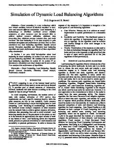
3.1. Random Unbiased Depth Probing The method starts by trivially dividing the tree into p subtrees with the purpose of estimating the average depth of each. This can be simply done by going down in the tree till finding a level that contains p subtrees. We consider the node count, as a function of depth, to represent a measure of the amount of work in each subtree; however, such function can be changed depending on application. To estimate the node count for each subtree, we perform a series of random depth probes to compute its average depth. Each probe randomly traverses the subtree from its root till hitting a leaf (terminating on a null child) and calculates the path length. A key issue with such sampling of leaves is its bias; the leaves that occur at shallow depths have much higher chances to be sampled than deeper ones. Fig. 1 shows two complete subtrees: Tree 1 and 2; the root of Tree 2 is joined on one of the leaves of Tree 1; the trees have n and m leaves, respectively. A random probe will visit a Tree 1’s leaf with probability 1/n; whereas it will visit a Tree 2’s leaf with probability 1/n × 1/m, resulting in biased sampling.
Tree 1 n leafs with prob. of access:
… 1/n 1/n
m leafs with prob. of access:
1/n
1/n
Tree 2 … 1/mn 1/mn
1/mn
Figure 1: Biased sampling
To resolve this issue, the obtained depths should be associated with weights; for two leaves separated by delta height of h, the upper leaf would have 2h more chance of being probed than the lower one. We, therefore, define a corresponding weight to normalize such effect. The weight wi for a depth d in a probe i is given by wi = w(di ) = 2di . Thus, at any probe, i, the weighted average for the i probes is given by: Pi k=1 dk wk (1) avgi = P i k=1 wk Algorithm 1 shows the process of computing the average node count of subtree. The subtree depth is calculated using the above formula for a series of i probes (lines 6:23). The corresponding node count is estimated as a function of depth. The running average count is effectively computed at each iteration to make the method more efficient (line 21). A sliding window of the last N counts (line 4) terminates probing based on a suitable probing stopping criteria (psc ) to be less than some threshold; in our implementation we adopt simple relative difference between the node count maximum and minimum values; however, other measures of variance can be used (such as absolute difference, standard deviation, . . . etc.). A simple node count estimator (exponential relation with depth, see Appendix A) is used as a fast way to terminate the algorithm, then a better estimator (Algorithm 2) is used for measuring the actual node count, based on Knuth [9], [10], when termination is reached. Algorithm 1 is repeated upon each subtree, preferably in parallel. Algorithm 2 is invoked at the return line of Algorithm 1; it takes the count of probes ending at each depth; The loop (lines 2-4) propagates the count up the levels so that recording the total number of times we visited that level. The next loop (lines 7-9) computes the number of nodes at each level by effectively multiplying the maximum number of nodes in the level by the ratio of visits to that level to
300
250
Cumulative Load (nodes)
the total number of visits (i.e. visits to root node), c(i)/c(1). The loops counts nodes for all levels, and returns. It is worth noting that the depth based estimator has a time complexity of O(n(da + b)) where n is the number of probes, d depth, a is the cost for one level traversal, and b is arithmetic operation cost. This is due to performing only one arithmetic operation per probe. Whereas using solely the Knuth-based estimator requires O(nd(a + b)) computations as every probe requires d arithmetic operations for each level traversal. Generally the cost of traversal is less than arithmetic operations, hence a