Hindawi Publishing Corporation Mathematical Problems in Engineering Volume 2016, Article ID 7473041, 13 pages http://dx.doi.org/10.1155/2016/7473041
Research Article An Efficient Method for Convex Constrained Rank Minimization Problems Based on DC Programming Wanping Yang, Jinkai Zhao, and Fengmin Xu School of Economics and Finance, Xi’an Jiaotong University, Xi’an 710061, China Correspondence should be addressed to Fengmin Xu;
[email protected] Received 26 January 2016; Revised 19 May 2016; Accepted 2 June 2016 Academic Editor: Srdjan Stankovic Copyright © 2016 Wanping Yang et al. This is an open access article distributed under the Creative Commons Attribution License, which permits unrestricted use, distribution, and reproduction in any medium, provided the original work is properly cited. The constrained rank minimization problem has various applications in many fields including machine learning, control, and signal processing. In this paper, we consider the convex constrained rank minimization problem. By introducing a new variable and penalizing an equality constraint to objective function, we reformulate the convex objective function with a rank constraint as a difference of convex functions based on the closed-form solutions, which can be reformulated as DC programming. A stepwise linear approximative algorithm is provided for solving the reformulated model. The performance of our method is tested by applying it to affine rank minimization problems and max-cut problems. Numerical results demonstrate that the method is effective and of high recoverability and results on max-cut show that the method is feasible, which provides better lower bounds and lower rank solutions compared with improved approximation algorithm using semidefinite programming, and they are close to the results of the latest researches.
1. Introduction In recent decades, with the increase of the system acquisition and data services, the explosion of data poses challenges to storage, transmission, and processing, as well as device design. The burgeoning theory of sparse recovery reveals the outstanding sensing ability on the large scales of highdimensional data. Recently, a new theory called compressed sensing (or compressive sampling (CS)) has appeared. And this theory is praised as a big deal in signal processing area. This approach can acquire the signals while compressing data properly. Its sampling frequency is lower than that of Nyquist, which makes the collections of high resolution signal possible. One noticeable merit of this approach is its ability to combine traditional data collection and data compression into a union when facing sparse representation signals. This merit means that sampling frequency of signals, time and computational cost consuming on data processing, and expense for data storage and transmission are all greatly reduced. Thus this approach leads signal processing to a new age. However, same with CS, Low Rank Matrix theory can also solve signal reconstruction problems that are related to theory and practice. It is also carried out through exerting
dimension reduction treatments on unknown multidimension signals validly. And then use sparse concepts in a more broad sense to the problems. That is to say, reconstruct the original high-dimensional signals array completely or approximately by a small number of values measured by sparse (or reducing dimensions) sampling. Considering that both of these two theories are closely related to intrinsic sparsity of signals, we generally view them as sparse recovery problems. The main goal of sparse recovery problems is using less linear measurement data to recovery high-dimensional sparse signal. Its core mainly includes three steps: signal sparse representation, linear dimension reduction measure, and the nonlinear reconstruction of signal. The three parts for the sparse recovery theory are closely related; each part will have a significant impact on the quality of signal reconstruction. However, the nonlinear reconstruction of signal can be seen as a special case of rank minimization problem to be solved. Constrained rank minimization problems have attracted a great deal of attention over recent years, which aim to find sparse solutions of a system. The problems are widely applicable in a variety of fields including machine learning [1, 2], control [3, 4], Euclidean embedding [5], image processing
2
Mathematical Problems in Engineering
[6], and finance [7, 8], to name but a few. There are some typical examples of constrained rank minimization problems; for example, one is affine matrix rank minimization problems [5, 9, 10] min
1 ‖A (𝑋) − 𝑏‖2𝐹 2
s.t.
rank (𝑋) ≤ 𝑘,
(1)
where 𝑋 ∈ 𝑅𝑚×𝑛 is the decision variable and the linear map A : 𝑅𝑚×𝑛 → 𝑅𝑝 and vector 𝑏 ∈ 𝑅𝑝 are known. Equation (1) includes matrix completion, based on affine rank minimization problem and compressed sensing. Matrix completion is widely used in collaborative filtering [11, 12], system identification [13, 14], sensor network [15, 16], image processing [17, 18], sparse channel estimation [19, 20], spectrum sensing [21, 22], and multimedia coding [23, 24]. Another is max-cut problems [25] in combinatorial optimization min
Tr (𝐿𝑋)
s.t.
diag (𝑋) = 𝑒 rank (𝑋) = 1
(2)
𝑋 ⪰ 0, where 𝑋 = 𝑥𝑥𝑇 , 𝑥 = (𝑥1 , . . . , 𝑥𝑛 )𝑇 , 𝐿 = (1/4)(diag(𝑊𝑒) − 𝑊), 𝑒 = (1, 1, . . . , 1)𝑇 , 𝑊 is the weight matrix, and so on. As a matter of fact, these problems can be written as a common convex constrained rank minimization model; that is, min 𝑓 (𝑋) s.t.
rank (𝑋) ≤ 𝑘
(3)
𝑋 ∈ Γ ∩ Ω, where 𝑓 : 𝑅𝑚×𝑛 → 𝑅 is a continuously differentiable convex function, rank(𝑋) is the rank of a matrix 𝑋, 𝑘 ≥ 0 is a given integer, Γ is a closed convex set, and Ω is a closed unitarily invariant convex set. According to [26], a set 𝐶 ⊆ 𝑅𝑛×𝑛 is a unitarily invariant set if {𝑈𝑋𝑉: 𝑈 ∈ 𝑈𝑚 , 𝑉 ∈ 𝑈𝑛 , 𝑋 ∈ 𝐶} = 𝐶,
(4)
where 𝑈𝑛 denotes the set of all unitary matrices in 𝑅𝑛×𝑛 . Various types of methods have been proposed to solve (3) or its special cases with different types of Γ ∩ Ω. When Γ ∩ Ω is 𝑅𝑚×𝑛 , (3) is the unconstrained rank minimization problem. One approach is to solve this case by convex relaxation of rank(⋅). Cai et al. [9] proposed singular value thresholding (SVT) algorithm; Ma et al. [10] proposed fixed point continuation (FPC) algorithm. Another approach is to solve rank constraint directly. Jain et al. [27] proposed simple and efficient algorithm Singular Value Projection (SVP) based on the projected gradient algorithm. Haldar and Hernando [28] proposed an alternating least squares approach. Keshavan et al. [29] proposed an algorithm based on optimization over a Grassmann manifold.
When Γ ∩ Ω is a convex set, (3) is a convex constrained rank minimization problem. One approach is to solve it by replacing rank constraint with other constraints, such as trace constraint and norm constraint. Based on this, several heuristic methods have been proposed in literature; for example, Nesterov et al. [30] proposed interior-point polynomial algorithms; Weimin [31] proposed an adaptive seminuclear norm regularization approach; in addition, semidefinite programming (SDP) has also been applied; see [32]. Another approach is to solve rank constraint directly. Grigoriadis and Beran [33] proposed alternating projection algorithms for linear matrix inequalities problems. Mohseni et al. [24] proposed penalty decomposition (PD) method based on penalty function. Gao and Sun [34] recently proposed the majorized penalty approach. Burer et al. [35] proposed nonlinear programming (NLP) reformulation approach. In this paper, we consider problem (3). We introduce a new variable and penalize equality constraints to objective function. By this technique, we can obtain closed-form solution and use it to reformulate the objective function in problem (3) as a difference of convex functions; then (3) is reformulated as DC programming which can be solved via linear approximation method. A function is called DC if it can be represented as the difference of two convex functions. Mathematical programming problems dealing with DC functions are called DC programming problems. Our method is different from original PD [26]; for one thing we penalize equality constraints to objective function and keep other constraints, while PD penalizes all except rank constraint to objective function, including equality and inequality constraints; for another each subproblem of PD is approximately solved by a block coordinate descent method, while we approximate problem (3) to a convex optimization to be solved finally. Compared with PD method, our method uses the closed-form solutions to remove rank constraint, while PD needs to consider rank constraint in each iteration. It is known that rank constraint is a nonconvex and discontinuous constraint, which is not easy to deal. And due to the remaining convex constraints, the formulated programming can be solved by solving a series of convex programming. In our method, we use linear function instead of the last convex function to formulate the programming to convex programming. We test the performance of our method by applying it to affine rank minimization problems and maxcut problems. Numerical results show that the algorithm is feasible and effective. The rest of this paper is organized as follows. In Section 1.1, we introduce the notation that is used throughout the paper. Our method is shown in Section 2. In Section 3, we apply it to some practical problems to test its performance. 1.1. Notations. In this paper, the symbol 𝑅𝑛 denotes the 𝑛dimensional Euclidean space, and the set of all 𝑚 × 𝑛 matrices with real entries is denoted by 𝑅𝑚×𝑛 . Given matrices 𝑋 and 𝑌 in 𝑅𝑚×𝑛 , the standard inner product is defined by ⟨𝑋, 𝑌⟩ fl Tr(𝑋𝑌𝑇 ), where Tr(⋅) denotes the trace of a matrix. The Frobenius norm of a real matrix 𝑋 is defined as ‖𝑋‖𝐹 fl √Tr(𝑋𝑋𝑇 ). ‖𝑋‖∗ denotes the nuclear norm of 𝑋, that is, the sum of singular values of 𝑋. The rank of a matrix 𝑋 is denoted
Mathematical Problems in Engineering
3
by rank(𝑋). We use 𝐼𝑞 to denote the identity matrix, whose dimension is 𝑞. Throughout this paper, we always assume that the singular values are arranged in nonincreasing order, that is, 𝜎1 ≥ 𝜎2 ≥ ⋅ ⋅ ⋅ ≥ 𝜎𝑟 > 0 = 𝜎𝑟+1 = ⋅ ⋅ ⋅ = 𝜎min{𝑚,𝑛} . 𝜕𝑓 denotes the subdifferential of the function 𝑓. We denote the adjoint of 𝐴 by 𝐴∗ . ‖𝐴𝐴𝑇 ‖(𝑘) is used to denote Ky Fan 𝑘-norms. Let 𝑃Ω be the projection onto the closed convex set Ω.
where 𝐷 = diag(𝜎1 , 𝜎2 , 𝜎3 , . . . , 𝜎𝑘 ) ∈ 𝑅𝑘×𝑘 . Thus, by the closed-form solution and the unitary invariance of 𝐹-norm, we have 𝜌 𝜌 𝑇 2 𝑈 𝑋𝑉 − 𝑈𝑇 𝑌𝑉 ‖𝑋 − 𝑌‖2𝐹 = min 𝐹 rank(𝑌)≤𝑘 2 rank(𝑌)≤𝑘 2 min
2. An Efficient Algorithm Based on DC Programming In this section, we first reformulated problem (3) as a DC programming problem with the convex constrained set, which can be solved via stepwise linear approximation method. Then, the convergence is provided. 2.1. Model Transformation. Let 𝑋 = 𝑌. Problem (3) is rewritten as
s.t.
𝑋 = 𝑌, rank (𝑌) ≤ 𝑘,
(5)
𝑋 ∈ Γ ∩ Ω. Adopting penalty function method to penalize 𝑋 = 𝑌 to objective function and choosing proper penalty parameter 𝜌, then (5) can be reformulated as
(6)
rank (𝑌) ≤ 𝑘, 𝑋 ∈ Γ ∩ Ω.
𝑋
s.t.
{𝑓 (𝑋) + min
𝜌
rank(𝑌)≤𝑘 2
‖𝑋 − 𝑌‖2𝐹 }
min 𝑓 (𝑋) +
𝜌 𝜌 𝑘 ‖𝑋‖2𝐹 − ∑𝜎𝑖2 (𝑋) 2 2 𝑖=1
(10)
𝑋 ∈ Γ ∩ Ω.
Clearly, 𝑓(𝑋) + (𝜌/2)‖𝑋‖2𝐹 is a convex function about 𝑋. Define function 𝑔 : 𝑅𝑚×𝑛 → 𝑅, 𝑔(𝑋) = ∑𝑘𝑖=1 𝜎𝑖2 (𝑋), 1 ≤ 𝑘 ≤ min{𝑚, 𝑛}. Next, we will study the property of 𝑔(𝑋). Problem (3) would be reformulated as a DC programming problem with convex constraints if 𝑔(𝑋) is a convex function, which can be solved via stepwise linear approximation method. In fact, it does hold, and 𝑔(𝑋) equals a trace function. Theorem 1. Let (11)
where 𝑂 denotes zero matrix whose dimension is determined depending on context; then, for any 𝑋 = 𝑈𝑆𝑉𝑇 ∈ 𝑅𝑚×𝑛 , the following hold:
(2) 𝑔(𝑋) = Tr(𝑋𝑇 𝑈𝑊𝑈𝑇 𝑋). (7)
𝑋 ∈ Γ ∩ Ω.
In fact, given the singular value decomposition, 𝑋 = 𝑈𝑆𝑉𝑇 , and singular values of 𝑋: 𝜎𝑗 (𝑋), 𝑗 = 1, . . . , min{𝑚, 𝑛}, where 𝑈 ∈ 𝑅𝑚×𝑚 and 𝑉 ∈ 𝑅𝑛×𝑛 are orthogonal matrices, the minimal optimal problem with respect to 𝑌 with 𝑋 fixed in (7), that is, minrank(𝑌)≤𝑘 (𝜌/2)‖𝑋 − 𝑌‖2𝐹 , has closed-form solution 𝑌 = 𝑈𝐶𝑉𝑇 with 𝐷 0 ), 𝐶=( 0 0
𝜌 𝜌 𝑘 ‖𝑋‖2𝐹 − ∑𝜎𝑖2 (𝑋) . 2 2 𝑖=1
(9)
(1) 𝑔(𝑋) is a convex function;
Solving 𝑌 with fixed 𝑋 ∈ Γ ∩ Ω, (6) can be treated as min
=
𝐼𝑘 𝑂 ) ∈ 𝑅𝑚×𝑚 , 𝑊=( 𝑂 𝑂
𝜌 min 𝑓 (𝑋) + ‖𝑋 − 𝑌‖2𝐹 2 s.t.
𝜌 ‖𝑆 − 𝐶‖2𝐹 2
Substituting the above into problem (7), problem (3) is reformulated as
s.t.
min 𝑓 (𝑋)
=
Proof. (1) Since {𝜎𝑗2 (𝑋) 𝑗 = 1, . . . , min(𝑚, 𝑛)} are eigenvalues
of 𝑋𝑋𝑇 , then 𝑔(𝑋) = ∑𝑘𝑖=1 𝜎𝑖2 (𝑋) = ‖𝑋𝑋𝑇 ‖(𝑘) , where ‖ ⋅ ‖(𝑘) is Ky Fan 𝑘-norms (defined in [36]). Clearly, ‖ ⋅ ‖(𝑘) is a convex function. Let 𝜑(⋅) = ‖ ⋅ ‖(𝑘) , 1 ≤ 𝑘 ≤ min{𝑚, 𝑛}. For ∀𝐴, 𝐵 ∈ 𝑅𝑚×𝑛 and 𝛼 ∈ [0, 1] we have 𝑔 (𝛼𝐴 + (1 − 𝛼) 𝐵) = 𝜑 ((𝛼𝐴 + (1 − 𝛼) 𝐵) (𝛼𝐴 + (1 − 𝛼) 𝐵)𝑇 ) = 𝜑 (𝛼2 𝐴𝐴𝑇 + 𝛼 (1 − 𝛼) 𝐴𝐵𝑇 + 𝛼 (1 − 𝛼) 𝐵𝐴𝑇 + (1 − 𝛼)2 𝐵𝐵𝑇 ) ≤ 𝛼2 𝜑 (𝐴𝐴𝑇 ) + 𝛼 (1 − 𝛼)
(8)
⋅ 𝜑 (𝐴𝐵𝑇 ) + 𝛼 (1 − 𝛼) 𝜑 (𝐵𝐴𝑇 ) + (1 − 𝛼)2 𝜑 (𝐵𝐵𝑇 ) .
(12)
4
Mathematical Problems in Engineering
Note that 𝐵𝐴𝑇 = (𝐴𝐵𝑇 )𝑇 ; thus they have the same nonzero singular values, and then 𝜑(𝐵𝐴𝑇 ) = 𝜑(𝐴𝐵𝑇 ) holds. Together with (12), we have 𝑇
𝜑 ((𝛼𝐴 + (1 − 𝛼) 𝐵) (𝛼𝐴 + (1 − 𝛼) 𝐵) ) ≤ 𝛼2 𝜑 (𝐴𝐴𝑇 ) + 2𝛼 (1 − 𝛼) 𝜑 (𝐴𝐵𝑇 )
(13)
+ (1 − 𝛼)2 𝜑 (𝐵𝐵𝑇 ) .
1 𝜎𝑗 (𝐴∗ 𝐵) ≤ 𝜎𝑗 (𝐴∗ 𝐴 + 𝐵∗ 𝐵) , 2
(14)
𝑘 𝑘 1 ∑ 𝜎𝑗 (𝐴𝑇 𝐵) ≤ ∑ 𝜎𝑗 (𝐴∗ 𝐴 + 𝐵∗ 𝐵) , 1 ≤ 𝑘 ≤ 𝑛. 𝑗=1 𝑗=1 2
(15)
That is, 1 𝜑 (𝐴𝐵𝑇 ) ≤ 𝜑 (𝐴𝐴𝑇 + 𝐵𝐵𝑇 ) , 2
s.t.
𝑘
𝑇
𝐹 (𝑋) = 𝑓 (𝑋) +
𝑘
𝑇
∑ 𝜎𝑗 (𝐴𝐴 + 𝐵𝐵 ) ≤ ∑𝜎𝑗 (𝐴𝐴 ) + ∑𝜎𝑗 (𝐵𝐵 ) . 𝑗=1
𝐻 (𝑋, 𝑋𝑖 ) = 𝑓 (𝑋) + (17) −
Thus 𝜑 (𝐴𝑇 𝐴 + 𝐵𝑇 𝐵) = 𝜑 (𝐴𝐴𝑇 + 𝐵𝐵𝑇 ) (18)
Together with (13) and (16), (18) yields 𝑔 (𝛼𝐴 + (1 − 𝛼) 𝐵) ≤ 𝛼𝜑 (𝐴𝐴𝑇 ) + (1 − 𝛼) 𝜑 (𝐵𝐵𝑇 ) = 𝛼𝑔 (𝐴) + (1 − 𝛼) 𝑔 (𝐵) .
(19)
Hence, 𝑔(𝑋) = ∑𝑘𝑖=1 𝜎𝑖2 (𝑋) is a convex function. (2) Let Θ = diag(𝜎1 , 𝜎2 , 𝜎3 , . . . , 𝜎𝑟 ) and 𝑟 is the rank of 𝑋, 𝑘≤𝑟 𝑆=(
Θ 𝑂 ) 𝑂 𝑂
𝜌 𝜌 ‖𝑋‖2𝐹 − Tr (𝑋𝑇 𝑈𝑊𝑈𝑇 𝑋) , 2 2
(20)
and we have
(24)
and the linear approximation function of 𝐹(𝑋) can be defined as
𝑗=1
≤ 𝜑 (𝐴𝐴𝑇 ) + 𝜑 (𝐵𝐵𝑇 ) .
(23)
2.2. Stepwise Linear Approximative Algorithm. In this subsection, we use stepwise linear approximation method [37] to solve reformulated model (23). Let 𝐹(𝑋) represent objective function of model (23); that is,
𝑇
𝑇
𝜌 𝜌 ‖𝑋‖2𝐹 − Tr (𝑋𝑇 𝑈𝑊𝑈𝑇 𝑋) 2 2
𝑋 ∈ Γ ∩ Ω.
(16)
where 𝐴𝐴 and 𝐵𝐵 are symmetric matrices. It is also known that, for arbitrary Hermitian matrices 𝐴𝐴𝑇 , 𝐵𝐵𝑇 ∈ 𝑅𝑚×𝑚 , 𝑘 = 1, 2, . . . , 𝑚, the following holds (see Exercise II.1.15 in [24])
𝑗=1
𝑇
Thus, Tr(𝑆 𝑊𝑆) = ∑𝑘𝑖=1 𝜎𝑖2 (𝑋) = 𝑔(𝑋) holds.
Since the objective function of (23) is a difference of convex functions, the constrained set Γ ∩ Ω is a closed convex constraint, so (23) is DC programming. Next, we will use stepwise linear approximate method to solve it.
Further,
𝑇
(22)
where Θ = diag (𝜎12 , 𝜎22 , 𝜎32 , . . . , 𝜎𝑘2 ).
min 𝑓 (𝑋) +
1 ≤ 𝑗 ≤ 𝑚, (see Theorem IX.4.2 in [36]) .
𝑘
𝑇
Θ 𝑂 Θ 𝑂 𝐼𝑘 𝑂 Θ 𝑂 𝑇 )=( ) ( )( ), 𝑆 𝑊𝑆 = ( 𝑂 𝑂 𝑂 𝑂 𝑂 𝑂 𝑂 𝑂
According to above theorem, (10) can be rewritten as
It is known that for arbitrary matrices 𝐴, 𝐵 ∈ 𝑅𝑚×𝑚 ,
𝑇
Moreover
𝜌 ‖𝑋‖2𝐹 2
𝜌 {𝑔 (𝑋𝑖 ) + ⟨𝜕𝑔 (𝑋𝑖 ) , 𝑋 − 𝑋𝑖 ⟩} , 2
(25)
where (𝜕𝑔(𝑋)/𝜕𝑋)(𝜕Tr(𝑋𝑇𝑈𝑊𝑈𝑇 𝑋)/𝜕𝑋) = 2𝑈𝑊𝑈𝑇 𝑋 (see 5.2.2 in [36]). Stepwise linear approximative algorithm for solving model (23) can be described as follows. Given the initial matrix 𝑋0 ∈ Γ ∩ Ω, penalty parameter 𝜌 > 0, rank 𝑘 > 0, 𝜏 > 1, set 𝑖 = 0. Step 1. Compute the single value decomposition of 𝑋𝑖 , 𝑈 𝑖 Σ𝑖 𝑉 𝑖 = 𝑋 𝑖 . Step 2. Update 𝑋𝑖+1 ∈ arg min {𝐻 (𝑋, 𝑋𝑖 )} 𝑋∈Γ∩Ω
(26)
Step 3. If stopping criterion is satisfied, stop; else set 𝑖 ← 𝑖 + 1 and 𝜌 ← (1 + 𝜏)𝜌 and go to Step 1. Remark
𝑇
Tr (𝑋𝑇 𝑈𝑊𝑈𝑇 𝑋) = Tr (𝑉𝑆 𝑈𝑇 𝑈𝑊𝑈𝑇 𝑈𝑆𝑉𝑇 ) 𝑇
𝑇
= Tr (𝑉𝑆 𝑊𝑆𝑉𝑇 ) = Tr (𝑆 𝑊𝑆) .
(21)
(1) Subproblem (26) can be done by solving a series of convex subproblems. The efficient method for convex programming is multiple and it has perfect theory guarantees.
Mathematical Problems in Engineering
5
(a) When Γ ∩ Ω is 𝑅𝑚×𝑛 , closed-form solutions can be obtained; for example, when solving model (1), 𝑋𝑖+1 = (𝐴∗ 𝐴 + 𝜌𝐼)−1 (𝜌𝑈𝑖 𝑊(𝑈𝑖 )𝑇 𝑋𝑖 ) are obtained by the first-order optimality conditions 𝑇
0 ∈ 𝜕𝑓 (𝑋) + 𝜌𝑋 − 𝜌𝑈𝑖 𝑊 (𝑈𝑖 ) 𝑋𝑖 .
𝑠
𝑘
𝑡
𝑘
𝑖=1
𝑖=1
𝑖=1
𝑖=1
= ∑𝜎𝑖2 − ∑𝜎𝑖2 + ∑𝛾𝑖2 − ∑𝛾𝑖2 𝑇
− 2 Tr (𝑌1𝑇 𝑌2 − 𝑌1 𝑌2 ) . (30)
(27)
(b) When Γ ∩ Ω is a general convex set, the closedform solution is hard to get, but subproblem (26) can be solved by some convex optimization software programs (such as CVX and CPLEX). According to different closed convex constraint sets, we can pick and choose suitable convex programming algorithm to combine with our method. The toolbox listed in this paper is just an alternative choice. (2) The stop rule that we adopted here is ‖𝑋𝑖+1 − 𝑋𝑖 ‖𝐹 ≤ 𝜀 with some 𝜀 small enough.
And we note that 𝑇
𝑇
Tr (𝑌1𝑇 𝑌2 − 𝑌1 𝑌2 ) = Tr ((𝑌1 − 𝑌1 ) (𝑌2 − 𝑌2 ) 𝑇
𝑇
+ (𝑌1 − 𝑌1 ) 𝑌2 + 𝑌1 (𝑌2 − 𝑌2 )) 𝑇
= Tr (𝑉1 (𝑆1 − 𝑊𝑆1 ) 𝑈1𝑇 𝑈2 (𝑆2 − 𝑊𝑆2 ) 𝑉2𝑇 𝑇
+ 𝑉1 (𝑆1 − 𝑊𝑆1 ) 𝑈1𝑇 𝑈2 𝑊𝑆2 𝑉2𝑇 + 𝑉1 (𝑊𝑆)
𝑇
𝑈1𝑇 𝑈2
(𝑆2 −
(31)
𝑊𝑆2 ) 𝑉2𝑇 )
𝑇
2.3. Convergence Analysis. In this subsection, we analyze the convergence properties of the sequence {𝑋𝑖 } generated by above algorithm. Before we prove the main convergence result, we give the following lemma which is analogous to Lemma 1 in [10]. Lemma 2. For any 𝑌1 and 𝑌2 ∈ 𝑅𝑚×𝑛 𝑌1 − 𝑌2 ≤ 𝑌1 − 𝑌2 𝐹 , 𝐹
(28)
diag (𝜎) 0 ) ∈ 𝑅𝑚×𝑛 𝑆1 = ( 0 0
(29)
diag (𝛾) 0 𝑆2 = ( ) ∈ 𝑅𝑚×𝑛 , 0 0
Next we estimate an upper bound for Tr(𝑌1𝑇𝑌2 − 𝑌1 𝑌2 ). According to Theorem 7.4.9 in [38], we get that an orthogonal matrix 𝑈 is a maximizing matrix for the problem max{Tr(𝐴𝑈): 𝑈 is orthogonal}, if and only if 𝐴𝑈 is positive semidefinite matrix. Thus, Tr((𝑆1 − 𝑊𝑆1 )𝑇 𝑈(𝑆2 − 𝑊𝑆2 )𝑉𝑇 ), Tr((𝑆1 − 𝑊𝑆1 )𝑇 𝑈𝑊𝑆2 𝑉𝑇 ), and Tr((𝑊𝑆)𝑇 𝑈(𝑆2 − 𝑊𝑆2 )𝑉𝑇 ) achieve their maximum, if and only if (𝑆1 − 𝑊𝑆1 )𝑇 𝑈(𝑆2 − 𝑊𝑆2 )𝑉𝑇 , (𝑆1 − 𝑊𝑆1 )𝑇 𝑈𝑊𝑆2 𝑉𝑇 , and (𝑊𝑆1 )𝑇 𝑈(𝑆2 − 𝑊𝑆2 )𝑉𝑇 are all positive semidefinite. It is known that when 𝐴𝐵 is positive semidefinite, Tr (𝐴𝐵) = ∑𝜎𝑖 (𝐴𝐵) ≤ ∑𝜎𝑖 (𝐴) 𝜎𝑖 (𝐵) . 𝑖
where 𝜎 = (𝜎1 , 𝜎2 , . . . , 𝜎𝑠 ), 𝜎1 ≥ ⋅ ⋅ ⋅ ≥ 𝜎𝑠 > 0 and 𝛾 = (𝛾1 , 𝛾2 , . . . , 𝛾𝑡 ), 𝛾1 ≥ ⋅ ⋅ ⋅ ≥ 𝛾𝑡 > 0. 𝑌𝑖 can be written as 𝑌𝑖 = 𝑈𝑖 𝑊𝑆𝑖 𝑉𝑖𝑇 , (𝑖 = 1, 2). Note that 𝑈1 , 𝑉1 , 𝑈2 , 𝑉2 are orthogonal matrices; we have 2 2 𝑌1 − 𝑌2 𝐹 − 𝑌1 − 𝑌2 𝐹
𝑖
(32)
Applying (32) to above three terms, we have 𝑇
Tr ((𝑆1 − 𝑊𝑆1 ) 𝑈 (𝑆2 − 𝑊𝑆2 ) 𝑉𝑇 ) ≤ ∑𝜎𝑖 (𝑆1 − 𝑊𝑆1 ) 𝜎𝑖 (𝑆2 − 𝑊𝑆2 ) 𝑖
𝑇
Tr ((𝑆1 − 𝑊𝑆1 ) 𝑈𝑊𝑆2 𝑉𝑇 )
𝑇
= Tr ((𝑌1 − 𝑌2 ) (𝑌1 − 𝑌2 ))
≤ ∑𝜎𝑖 (𝑆1 − 𝑊𝑆1 ) 𝜎𝑖 (𝑊𝑆2 )
𝑇
− Tr ((𝑌1 − 𝑌2 ) (𝑌1 − 𝑌2 ))
𝑖
𝑇
= Tr (𝑌1𝑇 𝑌1 − 𝑌1 𝑌1 + 𝑌2𝑇 𝑌2 − 𝑌2 𝑌2 ) 𝑇
𝑇
+ (𝑊𝑆1 ) 𝑈 (𝑆2 − 𝑊𝑆2 ) 𝑉𝑇 ) ,
𝑇
Proof. Without loss of generality, we assume 𝑚 ≤ 𝑛 and the singular value decomposition 𝑌1 = 𝑈1 𝑆1 𝑉1𝑇 𝑌2 = 𝑈2 𝑆2 𝑉2𝑇 with
− 2 Tr (𝑌1𝑇 𝑌2 − 𝑌1 𝑌2 )
𝑇
+ (𝑆1 − 𝑊𝑆1 ) 𝑈𝑊𝑆2 𝑉𝑇
where 𝑈 = 𝑈1𝑇 𝑈2 , 𝑉 = 𝑉1𝑇 𝑉2 are also orthogonal matrices.
where 𝑌𝑖 is the pre-𝑘 singular values approximate of 𝑌𝑖 (𝑖 = 1, 2).
𝑇
= Tr ((𝑆1 − 𝑊𝑆1 ) 𝑈 (𝑆2 − 𝑊𝑆2 ) 𝑉𝑇
𝑇
Tr ((𝑊𝑆1 ) 𝑈 (𝑆2 − 𝑊𝑆2 ) 𝑉𝑇 ) ≤ ∑𝜎𝑖 (𝑊𝑆1 ) 𝜎𝑖 (𝑆2 − 𝑊𝑆2 ) . 𝑖
(33)
6
Mathematical Problems in Engineering
Hence, without loss of generality, assuming 𝑘 ≤ 𝑠 ≤ 𝑡, we have 2 2 𝑌1 − 𝑌2 𝐹 − 𝑌1 − 𝑌2 𝐹 𝑠
𝑘
𝑡
𝑘
𝑠
≥ ∑𝜎𝑖2 − ∑𝜎𝑖2 + ∑𝛾𝑖2 − ∑𝛾𝑖2 − 2 ( ∑ 𝜎𝑖 𝛾𝑖 ) 𝑖=1
𝑖=1
𝑠
𝑖=1
𝑖=1
𝑖=𝑘+1
(34)
𝑡
2
= ∑ (𝜎𝑖 − 𝛾𝑖 ) + ∑ 𝛾𝑖2 ≥ 0
Proof. Assuming that 𝑋opt ∈ Υ is any optimal solution of problem (23) with Γ ∩ Ω = 𝑅𝑚×𝑛 , according to the first-order optimality conditions, we have 𝑇
0 = 𝜕𝑓 (𝑋opt ) + 𝜌𝑋opt − 𝜌𝑈opt 𝑊 (𝑈opt ) 𝑋opt .
𝑖=𝑠+1
𝑖=𝑘+1
Theorem 4. Let Υ be the set of stable points of problem (23) with no constraints; then the iterative sequence {𝑋𝑖 } generated by linear approximative algorithm converges to some 𝑋𝑜𝑝𝑡 ∈ Υ when 𝜌 → ∞.
Since 𝑋𝑖+1 ∈ arg min 𝑓(𝑋) + (𝜌/2)‖𝑋‖2𝐹 − (𝜌/2){𝑔(𝑋𝑖 ) + ⟨𝜕𝑔(𝑋𝑖 ), 𝑋 − 𝑋𝑖 ⟩}, then
which implies that ‖𝑌1 − 𝑌2 ‖𝐹 ≤ ‖𝑌1 − 𝑌2 ‖𝐹 holds. Next, we claim the value of iterations of stepwise linear approximative algorithm is nonincreasing. Theorem 3. Let {𝑋𝑖 } be the iterative sequence generated by stepwise linear approximative algorithm. Then {𝐹(𝑋𝑖 )} is monotonically nonincreasing.
𝑇
0 = 𝜕𝑓 (𝑋𝑖+1 ) + 𝜌𝑋𝑖+1 − 𝜌𝑈𝑖 𝑊 (𝑈𝑖 ) 𝑋𝑖 .
𝐻 (𝑋
𝑖
𝑖
𝑋𝑖+1 − 𝑋opt =
in which 𝑈opt 𝑊(𝑈opt )𝑇 𝑋opt − 𝑈opt 𝑊 ∑opt (𝑉opt )𝑇 − 𝑈𝑖 𝑊 ∑𝑖 (𝑉opt )𝑇 . By Lemma 2, we have
and 𝜕𝑔(𝑋) is the subdifferential of 𝑔(𝑋), which implies (36)
Let 𝑋 = 𝑋𝑖+1 , 𝑌 = 𝑋𝑖 in above inequality; we have 𝑔 (𝑋𝑖+1 ) ≥ 𝑔 (𝑋𝑖 ) + ⟨𝜕𝑔 (𝑋𝑖 ) , 𝑋𝑖+1 − 𝑋𝑖 ⟩ .
(37)
Therefore, 𝐻 (𝑋
𝑖+1
𝑖
, 𝑋 ) = 𝑓 (𝑋
𝑖+1
opt 𝑈 𝑊 (𝑈opt )𝑇 𝑋opt − 𝑈𝑖 𝑊 (𝑈𝑖 )𝑇 𝑋𝑖 𝐹 𝑖 opt opt opt 𝑇 𝑖 𝑖 𝑇 = 𝑈 𝑊 ∑ (𝑉 ) − 𝑈 𝑊 ∑ (𝑉 ) 𝐹 𝑖 opt ≤ 𝑋 − 𝑋 𝐹 .
=
(43)
𝑖+1 𝑋 − 𝑋opt = lim 𝑋𝑖+1 − 𝑋opt 𝐹 𝜌→∞ 𝐹 (38)
1 ≤ lim ( 𝜕𝑓 (𝑋𝑖+1 ) − 𝜕𝑓 (𝑋opt )𝐹 𝜌→∞ 𝜌 1 + 𝑋𝑖 − 𝑋opt 𝐹 ) = lim 𝜕𝑓 (𝑋𝑖+1 ) 𝜌→∞ 𝜌
= 𝐹 (𝑋𝑖+1 ) .
(44)
− 𝜕𝑓 (𝑋opt )𝐹 + lim 𝑋𝑖 − 𝑋opt 𝐹 = 𝑋𝑖 𝜌→∞
Consequently, 𝐹 (𝑋𝑖+1 ) ≤ 𝐻 (𝑋𝑖+1 , 𝑋𝑖 ) ≤ 𝐻 (𝑋𝑖 , 𝑋𝑖 ) = 𝐹 (𝑋𝑖 ) .
𝑈𝑖 𝑊(𝑈𝑖 )𝑇 𝑋𝑖
Norming both sides of (42), by the triangle inequalities property of norms, we have
𝜌 2 ) + 𝑋𝑖+1 𝐹 2
𝜌 − {𝑔 (𝑋𝑖 ) + ⟨𝜕𝑔 (𝑋𝑖 ) , 𝑋 − 𝑋𝑖 ⟩} 2 𝜌 2 𝜌 ≥ 𝑓 (𝑋𝑖+1 ) + 𝑋𝑖+1 𝐹 − 𝑔 (𝑋𝑖+1 ) 2 2
− 𝑈𝑖 𝑊 (𝑈𝑖 ) 𝑋𝑖
(35)
= 𝐹 (𝑋 ) ,
𝑔 (𝑋) ≥ 𝑔 (𝑌) + ⟨𝜕𝑔 (𝑌) , 𝑋 − 𝑌⟩ .
(42)
𝑇
𝑖
∀𝑋𝑌,
𝑇
, 𝑋 ) ≤ 𝐻 (𝑋 , 𝑋 ) 𝜌 2 𝜌 = 𝑓 (𝑋 ) + 𝑋𝑖 𝐹 − 𝑔 (𝑋𝑖 ) 2 2
1 (𝜕𝑓 (𝑋𝑖+1 ) − 𝜕𝑓 (𝑋opt )) 𝜌 + 𝑈opt 𝑊 (𝑈opt ) 𝑋opt
𝑖
𝑖
(41)
Equation (41) subtracts (40):
Proof. Since 𝑋𝑖+1 ∈ arg min{𝐻(𝑋, 𝑋𝑖 ) | 𝑋 ∈ Γ ∩ Ω}, we have 𝑖+1
(40)
(39)
We immediately obtain the conclusion as desired. Next, we show the convergence of iterative sequence generated by stepwise linear approximative algorithm when solving (23). Theorem 4 shows the convergence when solving (23) with Γ ∩ Ω = 𝑅𝑚×𝑛 .
− 𝑋opt 𝐹 , which implies that the sequence {‖𝑋𝑖 − 𝑋opt ‖𝐹 } is monotonically nonincreasing when 𝜌 → ∞. We then observe that {‖𝑋𝑖 − 𝑋opt ‖𝐹 } is bounded, and hence lim𝑖→∞ ‖𝑋𝑖 − 𝑋opt ‖𝐹 exists, denoted by ‖𝑋 − 𝑋opt ‖𝐹 , where 𝑋 is the limited point of {𝑋𝑖 }. Let 𝑖 → ∞ in (41); by the continuity, we get
Mathematical Problems in Engineering
7
𝑇
0 = 𝜕𝑓(𝑋) + 𝜌𝑋 − 𝜌𝑈𝑊𝑈 𝑋, which implies that 𝑋 ∈ Υ. By setting 𝑋 = 𝑋opt , we have
300
lim 𝑋𝑖 − 𝑋opt 𝐹 = 𝑋 − 𝑋opt 𝐹 = 0, 𝑖→∞
250
(45)
Now, we are ready to give the convergence of iterative sequence when solving (23) with general closed convex Γ∩Ω. Theorem 5. Let 𝜉 be the set of optimal solutions of problem (23); then the iterative sequence {𝑌𝑖 } generated by stepwise linear approximative algorithm converges to some 𝑌𝑜𝑝𝑡 ∈ 𝜉 when 𝜌 → ∞. Proof. Generally speaking, subproblem (26) can be solved by projecting a solution obtained via solving a problem with no constraints onto a closed convex set; that is, 𝑌𝑖+1 = 𝑃Γ∩Ω (𝑋𝑖+1 ), where 𝑋𝑖+1 ∈ arg min{𝐻(𝑋, 𝑋𝑖 )}. According to Theorem 4, the sequence {‖𝑋𝑖 − 𝑋opt ‖𝐹 } is monotonically nonincreasing and convergent when 𝜌 → ∞; together with the well known fact that 𝑃 is a nonexpansive operator, we have 𝑖 𝑌 − 𝑌opt = 𝑃Γ∩Ω (𝑋𝑖 ) − 𝑃Γ∩Ω (𝑋opt ) 𝐹 𝐹 𝑖 opt ≤ 𝑋 − 𝑋 𝐹 ,
(46)
where 𝑌opt is the projection of 𝑋opt onto Γ ∩ Ω. Clearly, 𝑌opt ∈ 𝜉. Hence, 0 ≤ lim𝑖→∞ ‖𝑌𝑖 − 𝑌opt ‖𝐹 ≤ lim𝑖→∞ ‖𝑋𝑖 − 𝑋opt ‖𝐹 = 0, which implies that 𝑌𝑖 converge to 𝑌opt . We immediately obtain the conclusion.
3. Numerical Results In this section, we demonstrate the performance of our method proposed in Section 2 by applying it to solve affine rank minimization problems (image reconstruction and matrix completion) and max-cut problems. The codes implemented in this section are written in MATLAB and all experiments are performed in MATLAB R2013a running Windows 7. 3.1. Image Reconstruction Problems. In this subsection, we apply our method to solve one case of affine rank minimization problems. It can be formulated as min
1 ‖A (𝑋) − 𝑏‖2𝐹 2
s.t.
rank (𝑋) ≤ 𝑘
(47)
𝑋 ∈ 𝑅𝑚×𝑛 , where 𝑋 ∈ 𝑅𝑚×𝑛 is the decision variable and the linear map A : 𝑅𝑚×𝑛 → 𝑅𝑝 and vector 𝑏 ∈ 𝑅𝑝 are known. Clearly, (47) is a special case of problem (3). Hence, our method can be suitably applied to (47). Recht et al. [39] have demonstrated that when we sample linear maps from a class of probability distributions, then they
SNR (dB)
200
which completes the proof.
150 100 50 0 600
800
1000 1200 1400 1600 1800 2000 2200 2400 The number of linear constraints
Gauss Binary
Sparse Binary Random Projection
Figure 1: Performance curves under four different measurement matrices: SNR versus the number of linear constraints.
would obey the Restricted Isometry Property. There are two ingredients for a random linear map to be nearly isometric. First, it must be isometric in expectation. Second, the probability of large distortions of length must be exponentially small. In our numerical experiments, we use four nearly isometric measurements. The first one is the ensemble with independent, identically distributed (i.i.d.) Gaussian entries. The second one has entries sampled from an i.i.d. symmetric Bernoulli distribution, which we call Bernoulli. The third one has zeros in two-thirds of the entries and others sampled from an i.i.d. symmetric Bernoulli distribution, which we call Sparse Bernoulli. The last one has an orthonormal basis, which we call Random Projection. Now we conduct numerical experiments to test the performance of our method for solving (47). To illustrate the scaling of low rank recovery for a particular matrix 𝑋, consider the MIT logo presented in [39]. The image has 46 rows and 81 columns (the total number of pixels is 46 × 81 = 3726). Since the logo only has 5 distinct rows, it has rank 5. We sample it using Gaussian i.i.d., Bernoulli i.i.d., Sparse Bernoulli i.i.d., and Random Projection measurements matrix with the number of linear constraints ranging between 700 and 2400. We declared MIT logo 𝑋 to be recovered if ‖𝑋 − 𝑋opt ‖𝐹 /‖𝑋‖𝐹 ≤ 10−3 ; that is, SNR ≥60 dB (SNR = −20 log(‖𝑋 − 𝑋opt ‖𝐹 /‖𝑋‖𝐹 )). Figures 1 and 2 show the results of our numerical experiments. Figure 1 plots the curves of SNR under four different measurement matrices mentioned above with different numbers of linear constraints. The numerical values on the 𝑥-axis represent the number of linear constraints 𝑝, that is, number of measurements, while those on 𝑦-axis represent the Signal to Noise Ration between the true original 𝑋 and 𝑋opt recovered by our method. Noticeably, Gauss and Sparse Binary can successfully reconstruct MIT logo images from about 1000 constraints, while Random Projection requires about
8
Mathematical Problems in Engineering 140
Table 1: DC versus SeDuMi in time (second). 𝑝 DC SeDuMi
120
SNR (dB)
100
800 46.82 93.26
900 50.49 120.16
1000 50.78 138.24
1100 51.38 159.44
1200 51.96 161.76
1500 54.09 245.38
80
sensitive to 𝑝 compared to SeDuMi. The reason is that closedform solutions can be obtained when we solve this problem. Comparisons are shown in Table 1.
60 40 20 0 700
800
900 1000 1100 1200 1300 1400 1500 The number of linear constraints
Gauss Binary
Sparse Binary Random Projection
Figure 2: Performance curves of nuclear norm heuristic method under four different measurement matrices: SNR versus the number of linear constraints.
1200 constraints. Binary requires the minimal constraints about 950. The Gauss and Sparse Binary measurements reach their maximal SNR of 220 dB at around 1500 constraints; the Binary measurements can reach its maximal SNR of 180 dB at around 1400 constraints. Random Projection has more large phase transition point but has the best recovery error. We observe a sharp transition to perfect recovery near 1000 measurements lower than 2𝑘(𝑚 + 𝑛 − 𝑘). Compared with Figure 2, which shows results of nuclear norm heuristic method in [39] and the method that is a kind of convex relaxations, there is a sharp transition to perfect recovery near 1200 measurements which is approximately equal to 2𝑘(𝑚 + 𝑛 − 𝑘). The comparison shows our method has better performance that it can recover an image with less constraints; namely, it needs less samples. In addition, we observe that SNR of nuclear norm heuristic method achieves 120 dB when the number of measurements approximately equals 1500, while our method just needs 1200 measurements, which decrease by 20% compared with 1500. If the number of measurements is 1500, accuracy of our method would be higher. Among precisions of four different measurement matrixes, the smallest one is precision of Random Projection. However, the precision value is also higher than 120 dB. The performance illustrates that our method is more accurate. Observing the curve of between 1200 and 1500, we can find that our curve rises smoothly compared with the curve in the same interval in Figure 2; this shows that our method is stable for reconstructing image. Figure 3 shows recovered images under four different measurement matrices with 800, 900, and 1000 linear constraints. And Figure 4 shows recovered images by our method and that by SeDuMi. We chose to use this interior-point method because it yields the highest accuracy. Distinctly, the recovered images by SeDuMi have some shadow, while ours is clear. Moreover, as far as time is concerned, our method is more fast and the computational time is not extremely
3.2. Matrix Completion Problems. In this subsection, we apply our method to matrix completion problems. It can be reformulated as min s.t.
1 2 𝑃 (𝑋) − 𝑃Ω (𝑀)𝐹 2 Ω rank (𝑋) ≤ 𝑘
(48)
𝑋 ∈ 𝑅𝑚×𝑛 , where 𝑋 and 𝑀 are both 𝑚 × 𝑛 matrices and Ω is a subset of index pairs (𝑖, 𝑗). Up to now, numerous methods were proposed to solve the matrix completion problem (see, e.g., [9, 10, 29, 31]). It is easy to see that problem (48) is a special case of general rank minimization problem (3) with 𝑓(𝑋) = (1/2)‖𝑃Ω (𝑋) − 𝑃Ω (𝑀)‖2𝐹 . In our experiments, we first created random matrices 𝑀𝐿 ∈ 𝑅𝑚×𝑘 and 𝑀𝑅 ∈ 𝑅𝑚×𝑘 with i.i.d. Gaussian entries and then set 𝑀 = 𝑀𝐿 𝑀𝑅𝑇 . We sampled a subset Ω of 𝑝 entries uniformly at random. We compare against singular value thresholding (SVT) method [9], FPC, FPCA [10], and the OptSpace (OPT) method [29] using 𝑃Ω (𝑋) − 𝑃Ω (𝑀)𝐹 ≤ 10−3 𝑃Ω (𝑀)𝐹
(49)
as a stop criterion. The maximum number of iterations is no more than 1500 in all methods; other parameters are default. We report result averaged over 10 runs. We use SR = 𝑝/(𝑚𝑛) to denote sampling ratio and FR = 𝑘(𝑚 + 𝑛 − 𝑘)/𝑝 to represent the dimension of the set of rank 𝑘 matrices divided by the number of measurements. NS and AT denote number of matrices that are recovered successfully and average times (seconds) that are successfully solved, respectively. RE represents the average relative error of the successful recovered matrices. We use the relative error ∗ 𝑀 − 𝑋 𝐹 \ ‖𝑀‖𝐹
(50)
to estimate the closeness of 𝑋∗ to 𝑀, where 𝑋∗ is the optimal solution to (48) produced by our method. We declared 𝑀 to be recovered if the relative error was less than 10−3 . Table 2 shows that our method has the close performance with OptSpace in column of NS. These performances are better than those of SVT, FPC, and FPCA. However, SVT, FPC, and FPCA cannot obtain the optimal matrix within 1500 iterations which shows that our method has advantage in finding the neighborhood of optimal solution. The results do not mean that these algorithms are invalid, but the maximum
Mathematical Problems in Engineering
9
Table 2: Numerical results for problems with 𝑚 = 𝑛 = 40 and SR = 0.5. Alg DC SVT FPC FPCA OptSpace DC SVT FPC FPCA OptSpace DC SVT FPC FPCA OptSpace DC SVT FPC FPCA OptSpace DC SVT FPC FPCA OptSpace
𝑘
FR
1
0.0988
2
0.1950
3
0.2888
4
0.3800
5
0.4688
NS 10 10 9 10 10 10 9 8 10 10 10 2 5 10 10 10 1 1 0 10 10 0 0 0 10
AT 0.02 0.11 0.13 0.03 0.01 0.03 0.18 0.14 0.02 0.01 0.05 0.36 0.25 0.06 0.04 0.06 0.62 0.25 — 0.05 0.08 — — — 0.09
RE 1.23𝐸 − 04 1.59𝐸 − 04 6.52𝐸 − 04 3.98𝐸 − 05 1.31𝐸 − 04 1.50𝐸 − 04 1.83𝐸 − 04 6.52𝐸 − 04 5.83𝐸 − 05 1.51𝐸 − 04 2.68𝐸 − 04 2.47𝐸 − 04 8.58𝐸 − 04 1.38𝐸 − 04 1.75𝐸 − 04 2.84𝐸 − 04 1.38𝐸 − 04 8.72𝐸 − 04 — 2.68𝐸 − 04 3.82𝐸 − 04 — — — 3.16𝐸 − 04
𝑘
FR
6
0.5550
7
0.6388
8
0.7200
9
0.7987
NS 9 0 0 0 10 9 0 0 0 9 7 0 0 0 9 4 0 0 0 4
AT 0.12 — — — 0.21 0.17 — — — 0.37 0.28 — — — 0.82 0.40 — — — 1.48
RA 4.64𝐸 − 04 — — — 4.05𝐸 − 04 6.11𝐸 − 04 — — — 5.37𝐸 − 04 7.90𝐸 − 04 — — — 6.68𝐸 − 04 8.93𝐸 − 04 — — — 9.28𝐸 − 04
AT 1.50 — — — 0.58 2.82 — — — 0.97 3.24 — — — 1.89
RA 5.05𝐸 − 04 — — — 5.57𝐸 − 04 7.45𝐸 − 04 — — — 6.57𝐸 − 04 7.66𝐸 − 04 — — — 7.95𝐸 − 04
Table 3: Numerical results for problems with 𝑚 = 𝑛 = 100 and SR = 0.2. Alg DC SVT FPC FPCA OptSpace DC SVT FPC FPCA OptSpace DC SVT FPC FPCA OptSpace DC SVT FPC FPCA OptSpace
𝑘
FR
1
0.0995
2
0.1980
3
0.2955
4
0.3920
NS 10 7 10 10 10 10 0 0 8 10 10 0 0 6 10 9 0 0 0 10
AT 0.30 1.82 3.14 0.12 0.03 0.77 — — 0.21 0.05 0.64 — — 0.09 0.12 1.16 — — — 0.22
RE 1.91𝐸 − 04 2.04𝐸 − 04 8.06𝐸 − 04 1.73𝐸 − 04 1.71𝐸 − 04 3.34𝐸 − 04 — — 2.97𝐸 − 04 2.27𝐸 − 04 3.03𝐸 − 04 — — 2.20𝐸 − 04 3.76𝐸 − 04 4.40𝐸 − 04 — — — 3.85𝐸 − 04
𝑘
FR
5
0.4875
6
0.5820
7
0.6755
NS 10 0 0 0 10 6 0 0 0 9 5 0 0 0 5
10
Mathematical Problems in Engineering
Figure 3: Recovered images under four measurement matrices with different numbers of linear constraints. From left to right: the original, results under Gauss, Binary, Sparse Binary, and Random Projection measurement. From top to bottom: 𝑝 = 800, 𝑝 = 900, and 𝑝 = 1000. Table 4: Numerical results for problems with 𝑚 = 𝑛 = 100 and SR = 0.3. Alg DC SVT FPC FPCA OptSpace DC SVT FPC FPCA OptSpace DC SVT FPC FPCA OptSpace DC SVT FPC FPCA OptSpace DC SVT FPC FPCA OptSpace DC SVT FPC FPCA OptSpace
𝑘
FR
1
0.0663
2
0.1320
3
0.1970
4
0.2613
5
0.3250
6
0.3880
NS 10 10 10 10 10 10 8 10 10 10 10 4 9 9 10 10 4 7 10 10 10 0 1 10 10 10 0 0 0 10
AT 0.19 0.68 1.33 0.17 0.05 0.20 1.39 2.18 0.16 0.04 0.25 1.77 4.32 0.19 0.07 0.32 9.82 5.02 0.18 0.09 0.37 — 8.18 0.10 0.19 0.47 — — 0.09 0.25
RE 1.49E − 04 1.66E − 04 4.47E − 04 6.12E − 05 1.29E − 04 1.69E − 04 1.66E − 04 4.84E − 04 7.68E − 05 1.48E − 04 1.92E − 04 1.23E − 04 5.82E − 04 1.21E − 04 1.98E − 04 2.30E − 04 4.67E − 04 6.59E − 04 6.63E − 04 2.08E − 04 2.72E − 04 — 7.34E − 04 2.20E − 04 2.67E − 04 3.00E − 04 — — 2.20E − 04 3.25E − 04
number of iterations is limited to 1500. When the rank of matrix is large (i.e., 𝑘 ≥ 5), the average time of our algorithm is less than that of OptSpace. In some cases, the relative errors of DC are minimal. When the dimension of matrix becomes larger, DC method has a better performance of NS and similar relative errors with that of OptSpace. In terms of time, our time is longer than that of OptSpace, but shorter than that of FPC and SVT. Tables 3 and 4 show the above results. In
𝑘
FR
7
0.4530
8
0.5120
9
0.5730
10
0.6333
11
0.6930
12
0.7520
NS 10 0 0 0 10 10 0 0 0 10 9 0 0 0 10 8 0 0 0 10 9 0 0 9 5 6 0 0 0 6
AT 0.61 — — — 0.47 0.87 — — — 0.63 1.03 — — — 1.40 1.36 — — — 1.80 2.19 — — — 4.11 2.83 — — — 6.44
RA 3.64E − 04 — — — 3.39E − 04 4.70E − 04 — — — 3.67E − 04 4.85E − 04 — — — 4.87E − 04 6.21E − 04 — — — 5.97E − 04 7.29E − 04 — — — 7.05E − 04 8.79E − 04 — — — 8.47E − 04
conclusion, our method has better performance in “hard” problems; that is, FR > 0.34. The problems involved matrices that are not of very low rank, according to [10]. Table 5 gives the numerical results for problems with large dimensions. In these numerical experiments, the maximum number of iterations is chosen by default of each compared method. We observe that our method can recover problems successfully as other four methods, while our method is
Mathematical Problems in Engineering
11 developed method for matrix completion problems while our method can be applied to more class of problems. To prove this, we will apply our method to max-cut problems. 3.3. Max-Cut Problems. In this subsection, we apply our method to max-cut problems. It can be formulated as follows: min Tr (𝐿𝑋) s.t.
Figure 4: Recovered images under different numbers of linear constraints. From left to right: the original, results under our method, and results by SeDuMi. From top to bottom: 𝑝 = 800, 𝑝 = 900, and 𝑝 = 1000.
Table 5: Numerical results for problems with different dimension. 𝑚(𝑛) 𝑘
𝑝
NS
AT
RA
100
10
DC SVT 0.57 0.34 FPC FPCA OptSpace
10 10 10 10 10
0.14 2.81 5.23 0.28 0.9
1.91E − 04 1.85E − 04 1.83E − 04 4.94E − 05 1.41E − 04
200
DC SVT 10 15665 0.39 0.25 FPC FPCA OptSpace
10 10 10 10 10
0.80 2.93 4.18 0.08 0.41
1.65E − 04 2.53E − 04 2.73E − 04 6.88E − 05 1.72E − 04
300
DC SVT 10 27160 0.30 0.22 FPC FPCA OptSpace
10 10 10 10 10
2.72 2.57 9.8 0.39 1.85
1.67E − 04 1.79E − 04 1.63E − 04 6.71E − 05 1.50E − 04
400
DC SVT 10 41269 0.26 0.19 FPC FPCA OptSpace
10 10 10 10 10
5.73 2.78 13.28 0.73 3.47
1.56E − 04 1.66E − 04 1.30E − 04 6.65E − 05 1.46E − 04
500
DC SVT 10 49471 0.20 0.2 FPC FPCA OptSpace
10 10 10 10 10
13.63 1.73E − 04 2.94 1.74E − 04 25.75 1.44E − 04 1.12 1.07E − 04 5.05 1.60E − 04
5666
SR
FR
Alg
DC SVT 1000 10 119406 0.12 0.17 FPC FPCA OptSpace
10 356.41 1.70E − 04 10 4.56 1.66E − 04 10 110.53 1.29E − 04 10 5.16 1.64E − 04 10 14.61 1.50E − 04
slower with the increase of dimension. However, our method is faster than FPC. Though SVT, FPCA, and OptSpace outperform our method in terms of speed, they are specifically
diag (𝑋) = 𝑒 rank (𝑋) = 1
(51)
𝑋 ⪰ 0, where 𝑋 = 𝑥𝑥𝑇, 𝑥 = (𝑥1 , . . . , 𝑥𝑛 )𝑇 , 𝐿 = (1/4)(diag(𝑊𝑒) − 𝑊), 𝑒 = (1, 1, . . . , 1)𝑇 , and 𝑊 is the weight matrix. Equation (51) is one general case of problem (3) with Γ ∩ Ω = {𝑋 | diag(𝑋) = 𝑒𝑋 ∈ 𝑆+ }. Hence, our method can be suitably applied to (51). We now address the initialization and termination criteria for our method when applied to (51). We set 𝑋0 = 𝑒𝑒𝑇 ; in addition, we choose the initial penalty parameter 𝜌 to be 0.01 and set the parameter 𝜏 to be 1.1. And we use ‖𝑋𝑖+1 − 𝑋𝑖 ‖𝐹 ≤ 𝜀 as the termination criteria with 𝜖 = 10−5 . In our numerical experiments, we first test several small scale max-cut problems; then we perform our method on the standard “𝐺” set problems written by Professor Ginaldi [40]. In all, we consider 10 problems ranging in size from 800 variables to 1000 variables. The results are shown in Tables 6 and 7, in which “𝑚” and “𝑘” represent corresponding dimension of graph and the rank of solution, respectively. The “obv” denotes objective values of optimal matrix solutions operated by our method. In Table 6, “KV” denotes known optimal objective values and “UB” presents upper bounds for max-cut by the semidefinite relaxation. It is easy to observe that our method is effective for solving these problems and it has computed the global optimal solutions of all problems. Moreover, we obtain lower rank solution compared with semidefinite relaxation method. Table 7 shows the numerical results for standard “𝐺” set problems. “SUB” denotes upper bounds by spectral bundle method proposed by Helmberg and Rendl [41]. “GW-cut” denotes the approximative algorithm proposed by Goemans and Williamson [42]. “DC” denotes results generated by our method, DC+ is the results of DC with neighborhood approximation algorithm, and the right most column, titled BK, gives best results as we have known according to [43, 44]. We use “—” to indicate that we do not obtain the rank. From Table 3 we can note that our optimal values are close to the results of latest researches, better than values given by GW-cut, and they are all less than the corresponding upper bounds. For the problems, we all get the lower rank solution compared with GW-cut; moreover, most solutions satisfy the constraints rank = 1. The results prove that our algorithm is effective when used to solve max-cut problems.
4. Concluding Remarks In this paper we used closed-form of penalty function to reformulate convex constrained rank minimization problems
12
Mathematical Problems in Engineering Table 6: Numerical results for famous max-cut problems.
Graph
𝑚
KV
C5 K5 AG BG
5 5 5 12
4 6 9.28 88
GW-cut UB 4.525 6.25 9.6040 90.3919
DC 𝑘 5 5 5 12
Table 7: Numerical results for G problems. Graph G01 G02 G03 G11 G14 G15 G16 G43 G45 G52
𝑚
SUB
800 800 800 800 800 800 800 1000 1000 1000
12078 12084 12077 627 3187 3169 3172 7027 7020 4009
GW-cut obv 𝑘 10612 14 10617 31 10610 14 551 30 2800 13 2785 70 2782 14 6174 — 6168 — 3520 —
DC obv 11281 11261 11275 494 2806 2767 2800 6321 6348 3383
𝑘 1 1 1 2 1 1 1 1 1 1
DC+
BK
11518 11550 11540 528 2980 2969 2974 6519 6564 3713
11624 11620 11622 564 3063 3050 3052 6660 6654 3849
as DC programming, which could be solved by stepwise linear approximative method. Under some suitable assumptions, we showed that accumulation point of the sequence generated by the stepwise linear approximative method was a stable point. The numerical results on affine rank minimization and max-cut problems demonstrate that our method is generally comparable or superior to some existing methods in terms of solution quality, and it can be applied to a class of problems. However, the speed of our method needs to be improved.
Competing Interests The authors declare that they have no competing interests.
Acknowledgments The authors need to acknowledge the fund projects. Wanping Yang and Jinkai Zhao are supported by Key Projects of Philosophy and Social Sciences Research (Ministry of Education, China, 15JZD012), Soft Science Fund of Shaanxi Province of China (2015KRM114), and the Fundamental Research Funds for the Central Universities. Fengmin Xu is supported by the Fundamental Research Funds for the Central Universities and China NSFC Projects (no. 11101325).
References [1] K.-C. Toh and S. Yun, “An accelerated proximal gradient algorithm for nuclear norm regularized linear least squares problems,” Pacific Journal of Optimization, vol. 6, no. 3, pp. 615–640, 2010.
obv 4 6 9.28 88
𝑘 1 1 1 1
Optimal solutions (−1; 1; −1; 1; −1) (−1; 1; −1; 1; −1) (−1; 1; 1; −1; −1) (−1; 1; 1; −1; −1; −1; −1; −1; −1; 1; 1; 1)
[2] Y. Amit, M. Fink, N. Srebro, and S. Ullman, “Uncovering shared structures in multiclass classification,” in Proceedings of the 24th International Conference on Machine Learning (ICML ’07), pp. 17–24, ACM, Corvallis, Ore, USA, June 2007. [3] L. El Ghaoui and P. Gahinet, “Rank minimization under LMI constraints: a framework for output feedback problems,” in Proceedings of the European Control Conference (ECC ’93), Gahinet P. Rank minimization under LMI constraints, Groningen, The Netherlands, June-July 1993. [4] M. Fazel, H. Hindi, and S. P. Boyd, “A rank minimization heuristic with application to minimum order system approximation,” in Proceedings of the IEEE American Control Conference (ACC ’01), vol. 6, pp. 4734–4739, Arlington, Va, USA, June 2001. [5] M. W. Trosset, “Distance matrix completion by numerical optimization,” Computational Optimization and Applications, vol. 17, no. 1, pp. 11–22, 2000. [6] B. Recht, M. Fazel, and P. A. Parrilo, “Guaranteed minimumrank solutions of linear matrix equations via nuclear norm minimization,” SIAM Review, vol. 52, no. 3, pp. 471–501, 2010. [7] L. Wu, “Fast at-the-money calibration of the libor market model through lagrange multipliers,” Journal of Computational Finance, vol. 6, no. 2, pp. 39–77, 2003. [8] Z. Zhang and L. Wu, “Optimal low-rank approximation to a correlation matrix,” Linear Algebra and its Applications, vol. 364, pp. 161–187, 2003. [9] J. F. Cai, E. J. Cand`es, and Z. Shen, “A singular value thresholding algorithm for matrix completion,” SIAM Journal on Optimization, vol. 20, no. 4, pp. 1956–1982, 2010. [10] S. Ma, D. Goldfarb, and L. Chen, “Fixed point and Bregman iterative methods for matrix rank minimization,” Mathematical Programming, vol. 128, no. 1-2, pp. 321–353, 2011. [11] K. Barman and O. Dabeer, “Analysis of a collaborative filter based on popularity amongst neighbors,” IEEE Transactions on Information Theory, vol. 58, no. 12, pp. 7110–7134, 2012. [12] S. T. Aditya, O. Dabeer, and B. K. Dey, “A channel coding perspective of collaborative filtering,” IEEE Transactions on Information Theory, vol. 57, no. 4, pp. 2327–2341, 2011. [13] N. E. Zubov, E. A. Mikrin, M. S. Misrikhanov, V. N. Ryabchenko, S. N. Timakov, and E. A. Cheremnykh, “Identification of the position of an equilibrium attitude of the international space station as a problem of stable matrix completion,” Journal of Computer and Systems Sciences International, vol. 51, no. 2, pp. 291–305, 2012. [14] T. M. Guerra and L. Vermeiren, “LMI-based relaxed nonquadratic stabilization conditions for nonlinear systems in the Takagi-Sugeno’s form,” Automatica, vol. 40, no. 5, pp. 823–829, 2004. [15] J. J. Meng, W. Yin, H. Li, E. Hossain, and Z. Han, “Collaborative spectrum sensing from sparse observations in cognitive radio networks,” IEEE Journal on Selected Areas in Communications, vol. 29, no. 2, pp. 327–337, 2011.
Mathematical Problems in Engineering [16] Z. Q. Dong, S. Anand, and R. Chandramouli, “Estimation of missing RTTs in computer networks: matrix completion vs compressed sensing,” Computer Networks, vol. 55, no. 15, pp. 3364–3375, 2011. [17] J. Wright, A. Y. Yang, A. Ganesh, S. S. Sastry, and Y. Ma, “Robust face recognition via sparse representation,” IEEE Transactions on Pattern Analysis and Machine Intelligence, vol. 31, no. 2, pp. 210–227, 2009. [18] H. Ji, C. Liu, Z. Shen, and Y. Xu, “Robust video denoising using Low rank matrix completion,” in Proceedings of the IEEE Computer Society Conference on Computer Vision and Pattern Recognition (CVPR ’10), pp. 1791–1798, San Francisco, Calif, USA, June 2010. [19] W. U. Bajwa, J. Haupt, A. M. Sayeed, and R. Nowak, “Compressed channel sensing: a new approach to estimating sparse multipath channels,” Proceedings of the IEEE, vol. 98, no. 6, pp. 1058–1076, 2010. [20] G. Taub¨ock, F. Hlawatsch, D. Eiwen, and H. Rauhut, “Compressive estimation of doubly selective channels in multicarrier systems: leakage effects and sparsity-enhancing processing,” IEEE Journal on Selected Topics in Signal Processing, vol. 4, no. 2, pp. 255–271, 2010. [21] Y. Tachwali, W. J. Barnes, F. Basma, and H. H. Refai, “The feasibility of a fast fourier sampling technique for wireless microphone detection in IEEE 802.22 air interface,” in Proceedings of the IEEE Conference on Computer Communications Workshops (INFOCOM ’02), pp. 1–5, IEEE, San Diego, Calif, USA, March 2010. [22] J. Meng, W. Yin, H. Li, E. Houssain, and Z. Han, “Collaborative spectrum sensing from sparse observations using matrix completion for cognitive radio networks,” in Proceedings of the IEEE International Conference on Acoustics, Speech, and Signal Processing (ICASSP ’10), pp. 3114–3117, Dallas, Tex, USA, March 2010. [23] S. Pudlewski and T. Melodia, “On the performance of compressive video streaming for wireless multimedia sensor networks,” in Proceedings of the IEEE International Conference on Communications (ICC ’10), pp. 1–5, IEEE, Cape Town, South Africa, May 2010. [24] A. H. Mohseni, M. Babaie-Zadeh, and C. Jutten, “Inflating compressed samples: a joint source-channel coding approach for noise-resistant compressed sensing,” in Proceedings of the IEEE International Conference on Acoustics, Speech, and Signal Processing (ICASSP ’09), pp. 2957–2960, IEEE, Taipei, Taiwan, April 2009. [25] S. J. Benson, Y. Ye, and X. Zhang, “Solving large-scale sparse semidefinite programs for combinatorial optimization,” SIAM Journal on Optimization, vol. 10, no. 2, pp. 443–461, 2000. [26] Z. Lu, Y. Zhang, and X. Li, “Penalty decomposition methods for rank minimization,” Optimization Methods and Software, vol. 30, no. 3, pp. 531–558, 2015. [27] P. Jain, R. Meka, and I. S. Dhillon, “Guaranteed rank minimization via singular value projection,” in Advances in Neural Information Processing Systems, pp. 937–945, 2010. [28] J. P. Haldar and D. Hernando, “Rank-constrained solutions to linear matrix equations using powerfactorization,” IEEE Signal Processing Letters, vol. 16, no. 7, pp. 584–587, 2009. [29] R. H. Keshavan, A. Montanari, and S. Oh, “Matrix completion from a few entries,” IEEE Transactions on Information Theory, vol. 56, no. 6, pp. 2980–2998, 2010.
13 [30] Y. Nesterov, A. Nemirovskii, and Y. Ye, Interior-Point Polynomial Algorithms in Convex Programming, Society for Industrial and Applied Mathematics, Philadelphia, Pa, USA, 1994. [31] M. Weimin, Matrix completion models with fixed basis coefficients and rank regularized problems with hard constraints [Ph.D. thesis], National University of Singapore, 2013. [32] M. Fazel, Matrix rank minimization with applications [Ph.D. thesis], Stanford University, 2002. [33] K. M. Grigoriadis and E. B. Beran, “Alternating projection algorithms for linear matrix inequalities problems with rank constraints,” in Advances in Linear Matrix Inequality Methods in Control, pp. 512–267, Society for Industrial and Applied Mathematics, Philadelphia, Pa, USA, 1999. [34] Y. Gao and D. Sun, “A majorized penalty approach for calibrating rank constrained correlation matrix problems,” 2010, http://www.math.nus.edu.sg/∼matsundf/MajorPen.pdf. [35] S. Burer, R. D. C. Monteiro, and Y. Zhang, “Maximum stable set formulations and heuristics based on continuous optimization,” Mathematical Programming, vol. 94, no. 1, pp. 137–166, 2002. [36] R. Bhatia, Matrix Analysis, Springer, Berlin, Germany, 1997. [37] Z. Lu, “Sequential convex programming methods for a class of structured nonlinear programming,” https://arxiv.org/abs/ 1210.3039. [38] R. A. Horn and C. R. Johnson, Matrix Analysis, Cambridge University Press, Cambridge, UK, 1985. [39] B. Recht, M. Fazel, and P. A. Parrilo, “Guaranteed minimumrank solutions of linear matrix equations via nuclear norm minimization,” SIAM Review, vol. 52, no. 3, pp. 471–501, 2010. [40] http://www.stanford.edu/∼yyye/yyye/Gset/. [41] C. Helmberg and F. Rendl, “A spectral bundle method for semidefinite programming,” SIAM Journal on Optimization, vol. 10, no. 3, pp. 673–696, 2000. [42] M. X. Goemans and D. P. Williamson, “Improved approximation algorithms for maximum cut and satisfiability problems using semidefinite programming,” Journal of ACM, vol. 42, no. 6, pp. 1115–1145, 1995. [43] G. A. Kochenberger, J.-K. Hao, Z. L¨u, H. Wang, and F. Glover, “Solving large scale max cut problems via tabu search,” Journal of Heuristics, vol. 19, no. 4, pp. 565–571, 2013. [44] G. Palubeckis and V. Krivickiene, “Application of multistart tabu search to the max-cut problem,” Information Technology and Control, vol. 31, no. 2, pp. 29–35, 2004.
Advances in
Operations Research Hindawi Publishing Corporation http://www.hindawi.com
Volume 2014
Advances in
Decision Sciences Hindawi Publishing Corporation http://www.hindawi.com
Volume 2014
Journal of
Applied Mathematics
Algebra
Hindawi Publishing Corporation http://www.hindawi.com
Hindawi Publishing Corporation http://www.hindawi.com
Volume 2014
Journal of
Probability and Statistics Volume 2014
The Scientific World Journal Hindawi Publishing Corporation http://www.hindawi.com
Hindawi Publishing Corporation http://www.hindawi.com
Volume 2014
International Journal of
Differential Equations Hindawi Publishing Corporation http://www.hindawi.com
Volume 2014
Volume 2014
Submit your manuscripts at http://www.hindawi.com International Journal of
Advances in
Combinatorics Hindawi Publishing Corporation http://www.hindawi.com
Mathematical Physics Hindawi Publishing Corporation http://www.hindawi.com
Volume 2014
Journal of
Complex Analysis Hindawi Publishing Corporation http://www.hindawi.com
Volume 2014
International Journal of Mathematics and Mathematical Sciences
Mathematical Problems in Engineering
Journal of
Mathematics Hindawi Publishing Corporation http://www.hindawi.com
Volume 2014
Hindawi Publishing Corporation http://www.hindawi.com
Volume 2014
Volume 2014
Hindawi Publishing Corporation http://www.hindawi.com
Volume 2014
Discrete Mathematics
Journal of
Volume 2014
Hindawi Publishing Corporation http://www.hindawi.com
Discrete Dynamics in Nature and Society
Journal of
Function Spaces Hindawi Publishing Corporation http://www.hindawi.com
Abstract and Applied Analysis
Volume 2014
Hindawi Publishing Corporation http://www.hindawi.com
Volume 2014
Hindawi Publishing Corporation http://www.hindawi.com
Volume 2014
International Journal of
Journal of
Stochastic Analysis
Optimization
Hindawi Publishing Corporation http://www.hindawi.com
Hindawi Publishing Corporation http://www.hindawi.com
Volume 2014
Volume 2014