An efficient method for transfer cross coefficient

An efficient method for transfer cross coefficient approximation in model based optical proximity correction Romuald Sabatiera,b , Caroline Fossatia , Salah Bourennanea and Antonio Di Giacomob a Institut Fresnel / Ecole ´ Centrale Marseille, CNRS UMR 6133 F-13397 Cedex 20, Marseille, France; b STM, 190 avenue C´ elestin Coq ZI 13106, Rousset, France ABSTRACT Model Based Optical Proximity Correction (MBOPC) is since a decade a widely used technique that permits to achieve resolutions on silicon layout smaller than the wave-length which is used in commercially-available photolithography tools. This is an important point, because masks dimensions are continuously shrinking. As for the current masks, several billions of segments have to be moved, and also, several iterations are needed to reach convergence. Therefore, fast and accurate algorithms are mandatory to perform OPC on a mask in a reasonably short time for industrial purposes. As imaging with an optical lithography system is similar to microscopy, the theory used in MBOPC is drawn from the works originally conducted for the theory of microscopy. Fourier Optics was first developed by Abbe to describe the image formed by a microscope and is often referred to as Abbe formulation. This is one of the best methods for optimizing illumination and is used in most of the commercially available lithography simulation packages. Hopkins method, developed later in 1951, is the best method for mask optimization. Consequently, Hopkins formulation, widely used for partially coherent illumination, and thus for lithography, is present in most of the commercially available OPC tools. This formulation has the advantage of a four-way transmission function independent of the mask layout. The values of this function, called Transfer Cross Coefficients (TCC), describe the illumination and projection pupils. Commonly-used algorithms, involving TCC of Hopkins formulation to compute aerial images during MBOPC treatment, are based on TCC decomposition into its eigenvectors using matricization and the well-known Singular Value Decomposition (SVD) tool. These techniques that use numerical approximation and empirical determination of the number of eigenvectors taken into account, could not match reality and lead to an information loss. They also remain highly runtime consuming. We propose an original technique, inspired from tensor signal processing tools. Our aim is to improve the simulation results and to obtain a faster algorithm runtime. We consider multiway array called tensor data T CC. Then, in order to compute an aerial image, we develop a lower-rank tensor approximation algorithm based on the signal subspaces. For this purpose, we propose to replace SVD by the Higher Order SVD to compute the eigenvectors associated with the different modes of TCC. Finally, we propose a new criterion to estimate the optimal number of leading eigenvectors required to obtain a good approximation while ensuring a low information loss. Numerical results we present show that our proposed approach is a fast and accurate for computing aerial images. Keywords: Optical lithography, Optical Proximity Correction, multiway array, signal subspace, Tensor signal processing

1. INTRODUCTION Model Based Optical Proximity Correction (MBOPC) can treat layouts by deforming mask pattern to improve resolution on silicon. As for current masks, several billions of segments have to be moved during several iterations necessary to reach convergence, fast and accurate algorithms are mandatory to perform OPC on a mask in a reasonable time for industry. To overcome this limitation, mathematical simplifications have to be done. As imaging with a lithography system

Photomask Technology 2008, edited by Hiroichi Kawahira, Larry S. Zurbrick, Proc. of SPIE Vol. 7122, 71221U · © 2008 SPIE · CCC code: 0277-786X/08/$18 · doi: 10.1117/12.801623

Proc. of SPIE Vol. 7122 71221U-1 2008 SPIE Digital Library -- Subscriber Archive Copy

(see Fig. 1) is analogous to microscopy, the theory used in MBOPC is drawn from works originally designed for microscopy theory. Fourier optics was first used to describe the image formed by a microscope.1, 2 In 1951, Hopkins developed an other formulation or method, equation (1), that has been afterward used in other works involving image formation.3–6 This formulation has the advantage of a four way transmission function independent of the shape of the object to image. However, this method, in aerial image computation for photolithography, remains highly runtime consuming and needs a numerical approximation in order to reach production constraints. A solution called Sum Of Coherent Systems (SOCS) provided by Cobb in7 consists into equation (2) matricization and decomposition into its eigenvectors, equation (3), allows to spare a huge amount of time while preserving a good accuracy as only the eigenvectors associated with the most energetic eigenvalues are used in calculus. Clearly, using Hopkins formulation, I(u, v)

=

1 2π

2 I2 I3 I4 I1 i1

i2

i3

T CC(i1 , i2 , i3 , i4 )E(i1 , i2 )E ∗ (i3 , i4 )ei{(i1 −i3 )u+(i2 −i4 )v} , (1)

i4

where +∞ T CC(i1 , i2 , i3 , i4 )

=

2π

Γ(x, y)F (x

+

i1 , y

+

i2 )F ∗ (x

+

i3 , y

+

i4 ) dx dy,

(2)

−∞

and I(.) E(.) Γ(.) F (.)

intensity image at the image plane. object being imaged (mask). mutual intensity function, describing coherence properties of the illumination. coherent point spread function, describing properties of the projection system.

Cobb has decomposed T CC into its eigenvectors yielding a matricized form, 2

T=

I

λk uk uH k .

(3)

k=1

Typically, I1 = I2 = I3 = I4 = I for non-astigmatic systems for symmetry reasons. In this article, In will denote the dimension of any n-mode of tensor T CC. This approximation describes the illumination and projection pupils. It can be thus calculated only once for a given imaging system. Nevertheless, runtime needed by existing algorithm SOCS can be improved using an other decomposition method. We propose thus to model data as a multiway array that we call a tensor. This approach allows to preserve interdimensional correlation avoiding possible data loss. A fixed point algorithm comes then replacing SVD algorithm to spare some computational load. The remainder of the paper is organized as follows: In section 2, some definition on tensors are proposed. Section 3 proposes an original lower rank tensor approximation (LRTA) adapted to TCC data approximation. In Section 4, we propose a runtime improvement algorithm using an original method. After presenting some experimental results in section 5, we conclude the paper in section 6. In the following, X will denote a tensor, X a matrix, x a vector and x a scalar.

Proc. of SPIE Vol. 7122 71221U-2

Illumination

Reticle — Object Plane

Diffraction Orders

Projection Optics Aerial Image

Plane Resist and Wafer Figure 1. General optical lithography process diagram.

2. TENSOR PROPERTIES 2.1 Tensor Definition The discretization of the four indices T CC in equation (2) and knowing the values of I1 , . . . , I4 are finite owing to Gamo’s previous work on matrix treatment of partial coherence.8 We can then write T CC as a four-way array, that we will call a tensor. Assuming we are working with spatially finite sources, γ is band limited as it represents the imaging source properties, T CC can be thus represented as a four-way data array, T CC. The interest of this representation is to approximate T CC without information loss due to inter-dimensional decorrelation implied by its matricization. In fact, subspace-based methods consider significant and remaining parts of the data, they are based on data most significant feature selection. Starting from signal realizations, subspace-based methods rely on second order statistics. In particular, the eigen-structure of the covariance matrix of signal realizations provides eigenvectors which span the measurement space. Within the measurement space, eigenvectors associated with the largest eigenvalues span the so-called “signal subspace”. Subspacebased methods are applied to source characterization in array processing, image denoising. Subspace-based methods were adapted to multidimensional -also called tensor- data.9 The tensor data extend the classical vector data.9 Tensor models were adopted in chemometrics,10, 11 for DS-CDMA system characterization,12 multi-linear independent component analysis,13 face recognition, signal processing,9 etc. In particular, subspacebased methods rely, for each mode, on the flattening matrix singular value decomposition and on data projection upon dominant singular vectors. Multidimensional filtering methods have been developed to consider data sets as whole entities. That is, the filtering keeps all inter-dimension relations while computation. The TUCKER3 decomposition14 has been used to compute higher order singular value decomposition (HOSVD)15 and lower rank(K1 , K2 , . . . , KN ) tensor approximation (LRTA-(K1 , K2 , . . . , KN )).16 This model has recently been applied in image processing for facial expression analysis and noise filtering of color images.9 Generally, we consider an N -order tensor to represent a multi-component array. Each of its elements are accessible through N indices (i1 , i2 , . . . , iN ). This tensor is written A ∈ RI1 ×...×IN , and each element ai1 ...iN . Each component is called an “n-mode” referring to the nth index of the tensor. A zero order tensor is a scalar, a first order tensor is a vector and a second order tensor is a matrix. To ease understanding this paper, some useful definitions are presented in the following.

2.2 Tensor Properties Here are given some tensor definitions:


• To study multi-way data properties in a particular n-mode direction, we define the n-mode flattening matrix of tensor A, written An ∈ RIn ×Mn where Mn = In+1 · · · I1 IN · · · In−1 .

Figure 2. Flattened matrix A2 ∈ RI2 ×I3 I1 in 2-mode of tensor A ∈ RI1 ×I2 ×I3 .

• ×n operator defines n-mode product. It generalizes matrix product to tensor and n-mode vector product in a particular n-mode. Consider tensor A ∈ RI1 ×...×IN and a matrix H(n) ∈ RJn ×In with In and Jn ∈ N∗ and ∀n ∈ {1, . . . , N }, n-mode product between A and H(n) is B = A ×n H(n) ∈ RI1 ×...In−1 ×Jn ×In+1 ...×IN . • Tensorial scalar product is defined as follows. Suppose two N order tensors: A and B ∈ RI1 ×...×IN . Scalar product between A and B is given by A|B = i1 ,...,iN ai1 ,...,iN bi1 ,...,iN . • Frobenius norm of a tensor A, written A is given by A = A|A = i1 ,...,iN a2i1 ,...,iN . • It is possible to define n-mode rank of a tensor as the generalization of column vectors line vectors rank of a matrix. n-mode rank of a tensor A ∈ RI1 ×...×IN , written Rankn (A), is the rank of flattened matrix An of A in n-mode, Rankn (A) = Rank(An ).

3. TENSOR APPROXIMATION BASED ON LRTA ALGORITHM As we intend to approximate the data tensor T CC for system transmission based on subspace algorithm (LRTA), we will consider in the following the four-way data tensor T CC ∈ RI1 ×···×I4 and the corresponding n-mode rank values by K1 , . . . , K4 . Assuming that the dimension Kn of the signal subspace is known for all n = 1 to N , see section 4.2 to know how to estimate them, one way to estimate the optimal approximation of tensor T CC, where T CC = T CC + E, (n) is to orthogonally project, for every n-mode, the vectors of tensor T CC on the nth-mode signal subspace E1 , 9, 12 for all n = 1 to 4. T CC = T CC ×1 P(1) ×2 P(2) ×3 P(3) ×4 P(4) .

(4)

In this last formulation, projectors P(n) are estimated owing to a multi-mode PCA applied to data tensor T CC. This multi-mode PCA-based approximation generalizes the classical matrix approximation methods.17–22 As a matter of fact, equation (3) can be rewritten to match equation (4): T = U Λ UH = Λ ×1 U ×2 U∗

(5)

In the vector or matrix formulation, the definition of the projector on the signal subspace is based on the eigenvectors associated with the largest eigenvalues of the covariance matrix of the set of observation vectors. Hence, the determination of the signal subspace amounts to determine the best approximation (in the leastsquares sense) of the observation matrix or the covariance matrix. As an extension to the vector and matrix cases, in the tensor formulation, the projectors on the nth-mode vector spaces are determined by computing the rank-(K1 , . . . , K4 ) approximation of T CC in the least-squares sense. From a mathematical point of view, the rank-(K1 , . . . , K4 ) approximation of T CC is represented by tensor


T CC K1 ,...,K4 which minimizes the quadratic tensor Frobenius norm T CC − B2 subject to the condition that B ∈ RI1 ×...×I4 is a rank-(K1 , . . . , K4 ) tensor. TUCKALS3 algorithm10, 23 is an optimal algorithm to estimate the different n-mode signal subspaces. The description of TUCKALS3 algorithm, used in rank-(K1 , . . . , K4 ) approximation is provided in Algorithm 1.

Algorithm 1 Lower Rank-(K1 , . . . , K4 ) Tensor Approximation (LRTA-(K1 , . . . , K4 )) 1. Input: data tensor T CC, and dimensions K1 , . . . , K4 of all n-mode signal subspaces. (n)

2. Initialization k = 0: For n = 1 to 4, calculate the projectors P0 (a) n-mode flatten T CC into matrix TCCn ;

given by HOSVD-(K1 , . . . , K4 ):

(b) Compute the SVD of TCCn ; (n)

(c) Compute matrix U0 formed by the Kn eigenvectors associated with the Kn largest singular values (n) of TCCn . U0 is the initial matrix of the n-mode signal subspace orthogonal basis vectors; (n)

(d) Form the initial orthogonal projector P0

(n)T

(n)

= U0 U0

on the n-mode signal subspace;

(e) Compute the HOSVD-(K1 , . . . , K4 ) of tensor T CC given by (1) (4) B0 = T CC ×1 P0 ×2 · · · ×4 P0 ; 2

3. ALS loop: Repeat until convergence, that is, for example, while Bk+1 − Bk > , > 0 being a prior fixed threshold, (a) For n = 1 to 4: (1)

(n−1)

(4)

i. Form B(n),k : B (n),k = T CC ×1 Pk+1 ×2 · · · ×n−1 Pk+1 ×n+1 · · · ×4 Pk ; (n),k

ii. n-mode flatten tensor B (n),k into matrix Bn (n),k

iii. Compute matrix C iv. Compute matrix (n)

of C(n),k . Uk iteration;

(n)

(n) Uk+1

;

(n),k Bn TCCTn ;

=

composed of the Kn eigenvectors associated with the Kn largest eigenvalues

is the matrix of the n-mode signal subspace orthogonal basis vectors at the k th (n)

(n)T

v. Compute Pk+1 = Uk+1 Uk+1 ; (1)

(4)

(b) Compute Bk+1 = T CC ×1 Pk+1 ×2 · · · ×4 Pk+1 ; (c) Increment k. (1) (4) CC 4. Output: the estimated signal tensor is obtained through T CC = T CC ×1 Pkstop ×2 · · · ×4 Pkstop . T is the rank-(K1 , . . . , K4 ) approximation of T CC, where kstop is the index of the last iteration after the convergence of TUCKALS3 algorithm.

In this algorithm, the second order statistics comes from the SVD of matrix TCCn at step 2b, which is equivalent, up to M1n multiplicative factor, to the estimation of tensor T CC n-mode vectors.9 The definition of Mn is given in (2.2). In the same way, at step 3(a)iii, matrix C(n),k is, up to M1n multiplicative factor, the estimation of the covariance matrix between tensor T CC and tensor B (n),k n-mode vectors. According to step 3(a)i, B (n),k represents data tensor T CC filtered in every mth-mode but the nth-mode, by projection-filters (m) Pl , with m = n, l = k if m > n and l = k + 1 if m < n. TUCKALS3 algorithm has recently been used to process a multi-mode PCA in order to perform white noise removal in color images.9 A good approximation of the rank-(K1 , . . . , K4 ) approximation can simply be achieved by computing the HOSVD-(K1 , . . . , K4 ) of tensor T CC.9, 15 Indeed, the HOSVD-(K1 , . . . , K4 ) of T CC consists of the initialization step of TUCKALS3 algorithm, and hence can be considered as a suboptimal solution for the rank-(K1 , . . . , K4 ) approximation of tensor T CC.15


This HOSVD-based technique has recently been used in9 for denoising and wave separation of multicomponent seismic data.

4. RUNTIME IMPROVEMENT: PROPOSED ALGORITHM 4.1 Fixed point algorithm We propose to adapt a Fixed Point algorithm24 to replace SVD in LRTA, algorithm 1, it allows to spare a high amount of computational load while preserving a high level of accuracy and has never been used in optical domain yet. One way to compute the K orthonormal basis vectors is to use Gram-Schmidt method (Algorithm 2). Algorithm 2 Fixed-point 1. Choose K, the number of principal axes or eigenvectors required to estimate. Consider matrix T and set p ← 1. 2. Initialize eigenvector up of size d × 1, e. g. randomly; 3. Update up as up ← Tup ; 4. Do the Gram-Schmidt orthogonalization process up ← up − 5. Normalize up by dividing it by its norm: up ←

j=p−1 j=1

(uTp uj )uj ;

up ||up || .

6. If up has not converged, go back to step 3. 7. Increment counter p ← p + 1 and go to step 2 until p equals K. The eigenvector with dominant eigenvalue will be measured first. Similarly, all the remaining K − 1 basis vectors (orthonormal to the previously measured basis vectors) will be measured one by one in a reducing order of dominance. The previously measured (p − 1)th basis vectors will be utilized to find the pth basis vector. The +T algorithm for pth basis vector will converge when the new value u+ p and old value up are such +Tthat up up = 1. It is usually economical to use a finite tolerance error to satisfy the convergence criterion up up − 1 < η where η is a prior fixed threshold. Let U = [u1 , u2 , . . . , uK ] be the matrix whose columns are the K orthonormal basis vectors. Then UUT is the projector onto the subspace spanned by the K eigenvectors associated with the largest eigenvalues. This subspace is also called “signal subspace”. It can be used in LRTA-(K1 , K2 , . . . , K4 ) to retrieve the basis vectors (n) U0 in step 2c of Algorithm 1. Thus, the initialization step is faster since it does not need the In basis vectors but only the Kn first ones and it does not need the step 2b, i.e. SVD of the data tensor n-mode flattening matrix TCCn . According to what have been explained above, fixed point algorithm will replace SVD in LRTA algorithm, in order to improve runtime. However, a prerequisite to this algorithm is the knowledge of each n-mode rank. A method to determine them is developed in next subsection.

4.2 n-mode rank estimation Whereas a common way to obtain K1 . . . K4 values is to use empirical data,25 we wish to present here a scientific tool optimizing the calculation. Each projector P(n) , n = 1 · · · 4 is estimated by the truncation of flattening matrices TCCn using SVD. That is, by keeping the Kn eigenvectors associated with the Kn highest singular values of TCCn , n = 1, . . . , 4. In order to estimate the signal subspace dimension for each n-mode, we extend the well-known detection criterion.26 Thus, the optimal signal subspace dimension is obtained merely by minimizing one of AIC27 or MDL28 criteria.


Consequently, for each n-mode unfolding of T CC, the form of detection criterion AIC can be expressed as G(λk+1 , . . . , λp ) + 2k(2p − k) A(λk+1 , . . . , λp )

(6)

1 G(λk+1 , . . . , λp ) + k(2p − k) ln N A(λk+1 , . . . , λp ) 2

(7)

AIC(k) = −2(p − k)N ln and the MDL criterion is given by

M DL(k) = −(p − k)N ln

where G and A are geometric and arithmetic mean respectively. (λi )1≤i≤In are In eigenvalues of the covariance matrix of the n-mode unfolding T CC: λ1 ≥ λ2 ≥ . . . ≥ λIn , and N is the number of columns of the n-mode unfolding T CC. The n-mode rank Kn is the value of k (k = 1, . . . , In − 1) which minimizes AIC or MDL criterion.

5. EXPERIMENTAL RESULTS The proposed methods can be applied to any multidimensional data set such as image, multicomponent seismic signals, hyper-spectral images. . We wish to compare LRTA algorithm benefits over SOCS algorithm. We use square size matrices with increasing rows and columns number as data set to compare algorithms runtime and accuracy.

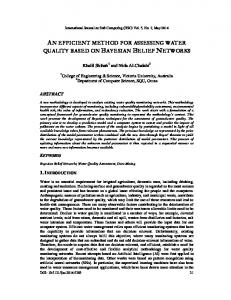
5.1 Runtime improvement We first focus on Fixed Point algorithm runtime gain toward SVD algorithm. Figure 3 shows runtime curves of increasing size matrices decomposition. Matlab SVD algorithm is used. We chose to compute 10 eigenvectors for each matrix with fixed point algorithm. This value corresponds to an average value of eigenvectors number used in classical OPC models. However, as Fixed Point algorithm runtime is linear with eigenvectors number to compute, Table 1 shows that this number can be increased up to around 300 eigenvectors for 3000 × 3000 matrices and up to around 100 eigenvectors for 120 × 120 matrices.

Runtime Comparison between Fixed Point and SVD 500

Fixed Point

-

400

-t300

/ ------SVD

-

7-

c'

200 100

-

0

0

500

I

I

I

I

1000

1500

2000

2500

3000

Square Matrix Size

Figure 3. Computational times (in sec.) as a function of rows and columns number.


Matrix size SVD runtime (sec) Fixed point runtime (sec) SVD/FP rate

120 0,109 0,010 10,629

720 6,262 0,406 15,441

1320 38,911 1,762 22,083

1920 122,810 4,536 27,073

2520 279,762 9,220 30,343

3000 489,808 14,522 33,728

Table 1. Some numerical values corresponding with Figure 3.

5.2 Fixed Point algorithm reconstruction error In order to assess our algorithm precision toward SVD decomposition, Figure 4 shows reconstruction error of T−T both Fixed Point and SVD algorithms, T , where T denotes the original matrix and T the reconstructed matrix. For constancy purposes with Fixed Point algorithm, only the 10 first eigenvectors computed with SVD are used for reconstruction. Reconstruction Error Comparison between Fixed Point and svD 0,12

0! 0!04 0,02

0

500

1000

1500

2000

2500

3000

Square Matrix Size

Figure 4. Reconstruction error comparison between SVD and Fixed Point Algorithm.

5.3 AIC and MDL criteria Figure 5 shows AIC and MDL functions of a fourth order tensor filled with random data. The minimum value in AIC and MDL curves gives rank estimation value of considered mode.

5.4 Comparison between LRTA and SOCS algorithms Figure 6 shows a comparison of SOCS and LRTA algorithms reconstruction error. To obtain these curves, random tensors of increasing size have been created. They have been unfolded following Cobb’s method,7 decomposed using SVD algorithm, recomposed using only the dominant eigenvectors. In the same time, they have been decomposed using LRTA algorithm and also recomposed using only the dominant eigenvectors. In both cases, the error function is the same than used in subsection 5.2 to compute fixed point algorithm vs. SVD algorithm error. The curves show clearly the benefit of our method which, as announced, takes advantage of interdimensional correlation, avoiding data loss induced by matricization. The computations have been run with Matlab on a 2.4GHz dual core Pentium with 4Go RAM under Windows XP .


0

50

100

200 250 Eigenvalues indices

150

300

40

350

Both criteria evolution as a function of ei genvalues

1

AIC

MDL

50

100

150

200

250

300

350

400

Ranks

Figure 5. Comparison of rank mode estimation using AIC and MDL criteria.

SOCS vs. LRTA error 0.

Input size

Figure 6. Comparison of LRTA and SOCS reconstruction error.


6. CONCLUSION We have proposed here a new approach to Transfer Cross Coefficients data set approximation in diffraction theory of optical images based on multi-linear algebra tools. The goal of this work is two way axed, it allows to adapt complex physical equations to tensor computation and to improve runtime by using fixed point algorithm instead of HOSVD while preserving accuracy by using LRTA and AIC algorithm. We have proven our method to be faster and more accurate than existing SOCS method, as we obtain a lower reconstruction error than SOCS algorithm, whatever the size of input data is. Those methods have proven their efficiency in other domains, such as multidimensional images restoration or denoising and for wave separation of multicomponent seismic data, but have never been implemented in imaging theory yet. In further work, we will bring more detailed experimental data to express in real cases the extent of the improvement of our method.

REFERENCES 1. 2. 3. 4. 5. 6. 7. 8. 9. 10. 11. 12. 13. 14. 15. 16. 17. 18. 19. 20. 21. 22. 23.

Hecht, E., [Optics], Addison-Wesley Publishing, Massachussetts (1987). Goodman, J., [Introduction to Fourier optics], McGraw-Hill, New York (1996). Hopkins, H., “The concept of partial coherence in optics,” Proc. Royal Soc. Series A 208, 263–277 (1951). Hopkins, H., “On the diffraction theory of optical images,” Proc. Royal Soc. Series A 217(1131), 408–432 (1952). Born, M. and Wolf, E., [Principles of Optics], pergamon press ed. (1980). Flanner, P., “Two-dimensional optical imaging for photolithography simulation,” Technical Report Memorandum (Jul 1986). Cobb, N., Fast Optical and Process Proximity Correction Algorithms for Integrated Circuit Manufacturing, phD thesis, University of California at Berkeley (1998). Gamo, H., [Progress in Optics], vol. 3, North-Holland Publishing Company, e. wolf ed. (1964). chapter 3: Matrix Treatment of Partial Coherence. Muti, D. and Bourennane, S., “Survey on tensor signal algebraic filtering,” Signal Processing (87), 237–249 (2007). Sidiropoulos, N. and Bro, R., “On the uniqueness of multilinear decomposition of N-way arrays,” Journal of Chemometrics 14, 229–239 (2000). Kiers, H., “Towards a standardized notation and terminology in multiway analysis,” Journal of Chemometrics 14, 105–122 (2000). Lathauwer, L. and Castaing, J., “Tensor-based techniques for the blind separation of DS-CDMA signals,” Signal Processing 87(2), 322–336 (2007). Vasilescu, M. and Terzopoulos, D., “Multilinear independent components analysis,” Proc. IEEE Conf. on Computer Vision and Pattern Recognition (CVPR’05) 1, 547–553 (06 2005). Tucker, L., “Some mathematical notes on three-mode factor analysis,” Psychometrika 31, 279–311 (1966). Lathauwer, L., Moor, B. D., and Vandewalle, J., “A multilinear singular value decomposition,” SIAM Jour. on Matrix An. and Applic. 21, 1253–78 (2000). Lathauwer, L. and Vandewalle, J., “Dimensionality reduction in higher-order signal processing and rank(r1 , r2 , ..., rn ) reduction in multilinear algebra,” Linear Algebra and its Applications 391, 31–55 (2004). Freire, F. and Ulrych, T., “Application of SVD to vertical seismic profiling,” Geophysics 53, 778–785 (1988). Glangeaud, F. and Mari, J., [Wave separation], Technip IFP ed. (1994). Hemon, M. and Mace, D., “The use of Karhunen-Loeve transform in seismic data prospecting,” Geophysical Prospecting 26, 600–626 (1978). Hsu, K., “Wave separation and feature extraction of accoustic well-logging waveforme of triaxial recordings by singular value decomposition,” Geophysics 55, 176–184 (1990). Jackson, G., Mason, I., and Greenhalgh, S., “Principal component transforms of triaxial recordings by singular value decomposition,” Geophysics 56(4), 176–184 (1991). Liu, X., “Ground roll suppression using the Karhunen-Loeve transform,” Geophysics 64(2), 564–566 (1991). Kiers, H., “Towards a standardized notation and terminology in multiway analysis,” Journal of Chemometrics 14, 105–122 (2000).


24. Hyv˝ arinen, A. and Oja, E., “A fast-fixed point algorithm for independent component analysis,” Neural comput. 9(7), 1483–1492 (1997). 25. Zuniga, C. and Tejnil, E., “Heuristics for truncating the number of kernels in hopkins,” in [SPIE Advanced Lithography], (2007). 26. Wax, M. and Kailath, T., “Detection of signals information theoretic criteria,” IEEE Trans. on Acoust., Speech, Signal Processing 33, 387–392 (April 1985). 27. Akaike, H., “A new look at the statistical model identification,” IEEE Trans. on automatic control 19(6), 716–723 (1974). 28. Rissanen, J., “A universal prior for integers and estimation by minimum description length,” The Annals of Statistics 11(2), 416–431 (1983).
