AN EFFICIENT MODAL FDTD FOR ABSORBING BOUNDARY ... - PIER

Progress In Electromagnetics Research, PIER 68, 229–246, 2007

AN EFFICIENT MODAL FDTD FOR ABSORBING BOUNDARY CONDITIONS AND INCIDENT WAVE GENERATOR IN WAVEGUIDE STRUCTURES S. Luo and Z. Chen Department of Electrical and Computer Engineering Dalhousie University 1360 Barrington Street, Halifax, NS, B3J 1Z1, Canada Abstract—When the finite-difference time-domain method is used to compute waveguide structures, incident waves are needed for calculating electrical parameters (e.g., the scattering parameters), and effective absorbing boundary conditions are required for terminating open waveguide structures. The incident waves are conventionally obtained with inefficient three-dimensional (3D) simulations of long uniform structures, while the absorbing boundary conditions reported so far do not perform well at or below cut-off frequencies. To address the problems, we propose a novel one-dimensional (1D) finitedifference time-domain method in this paper. Unlike the other methods developed so far, the proposed method is derived from the finite-difference time-domain formulation, and therefore has the same numerical characteristics as that of the finite-difference time-domain method. As a result, when used to obtain an incident wave, it produces results almost identical to those produced by the conventional finitedifference time-domain method except computer rounding-off errors. When used as the absorbing boundary condition, it produces reflections of less than −200 dB in entire frequency spectrum including the cut-off frequencies. 1. INTRODUCTION Since the finite-difference time-domain (FDTD) method was reported [1], it has become a popular numerical method in solving Maxwell’s equations because of its simplicity and flexibility [2]. The FDTD method has been applied to compute waveguide structures. To do so, two things are often needed: a known incident wave for calculating electrical parameters (e.g., scattering parameters) and an effective absorbing boundary condition for terminating open structures.

230

Luo and Chen

To obtain an incident wave, a separate simulation of a long waveguide structure usually is run [3]. For a 3D structure, such a simulation is often inefficient because the simulation is executed in three dimensions and therefore requires large memory and CPU time. In order to solve the problems as well as to develop efficient absorbing boundary conditions, many 1D modal absorbing boundary conditions (modal ABCs) have been proposed [4–14]. Most of them use analytically or numerically generated Green’s functions or impedance functions. However, these Green’s functions or impedance functions often have numerical characteristics different from those of 3D FDTD formulations, especially for frequencies around the cut-off frequency of a waveguide mode. Consequently, they do not offer highly accurate results, for instance, near or below the cut-off frequency of a waveguide mode. To resolve the problem, we propose a new compact 1D FDTD method in this paper. Unlike other methods reported so far, this method is derived directly from the FDTD formulations; therefore, it has the same numerical characteristics as that of the 3D FDTD method with which it interfaces. As a result, it not only allows efficient computation of an incident wave due to its one dimensional nature, but also provides a truly perfect modal absorbing boundary conditions (modal ABCs) (better than −200 dB for the full frequency spectrum, including the cut-off frequency). The preliminary work on the method was reported in [15] while this paper presents the full developments and thorough studies for the method, including dispersion analysis (that rationalizes the excellence performance of the method) and more numerical tests. In other words, in modeling a long uniform waveguide structure, the proposed 1D method can be used to replace the conventional 3D FDTD method with much higher efficiency and the other existing methods with at least much better accuracy and performance. Note that since the accuracy and validity of conventional 3D FDTD method have been studied and proven in the past four decades, its results are used in this paper as the benchmark solutions for comparisons with the proposed method. This paper is organized as follows. Section 2 presents the derivation of the proposed 1D method. Section 3 shows the dispersion analysis of the proposed method. Section 4 describes the two applications of the proposed method: generation of the incident wave and absorption of waves. Section 4 presents the numerical results that demonstrate the validity and effectiveness of the proposed technique. Further discussion and conclusions relating to the proposed method follow in Section 5.

Progress In Electromagnetics Research, PIER 68, 2007

231

2. FORMULATION OF THE PROPOSED 1D FDTD METHOD The conventional 3D FDTD formulations, which are well-known, contain computations that are recursive in time [2]. For instance, for Ex and Hy , = Ex |ni− 1 , j, k Ex |n+1 i− 12 , j, k 2   ∆t n+ 12 n+ 12 + Hz |i− 1 , j+ 1 , k − Hz |i− 1 , j− 1 , k ε∆y 2 2 2 2   1 1 ∆t n+ 2 n+ 2 Hy |i− 1 , j, k+ 1 − Hy |i− 1 , j, k− 1 − ε∆z 2 2 2 2 n+ 1

(1a)

n− 1

Hy |i− 12, j, k− 1 = Hy |i− 12, j, k− 1 2 2 2 2  ∆t  n Ez |i, j, k− 1 − Ezn |ni−1, j, k− 1 + 2 2 µ∆x  ∆t  n n − Ex |i− 1 , j, k − Exn |ni− 1 , j, k−1 2 2 µ∆z

(1b)

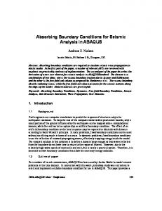
The equations for the other field components can be expressed similarly. For a homogeneously filled waveguide, field distributions of a given mode on a cross-section do not change with time, frequency and the longitudinal coordinate. They can be found analytically or numerically (e.g., [16, 17]). Suppose that a mode is traveling in z-direction and Yee’s grid is applied as shown in Fig. 1. The fully discretized Maxwell’s equations (1) can then be rewritten as: = Ex |ni− 1 , j, k Ex |n+1 i− 12 , j, k 2  ∆t  n+ 1 αzy |i− 1 , j− 1 − 1 Hz |i− 12, j− 1 , k + 2 2 ε∆y 2 2   1 ∆t n+ 2 n+ 12 Hy |i− 1 , j, k+ 1 − Hy |i− 1 , j, k− 1 − ε∆z 2 2 2 2 n+ 1

(2a)

n− 1

Hy |i− 12, j, k− 1 = Hy |i− 12, j− 1 , k− 1 2

2

2

2

2

∆t + (1 − βzx |i, j ) Ez |ni, j, k− 1 2 µ∆x  ∆t  n − Ex |i− 1 , j, k − Ex |ni− 1 , j, k−1 2 2 µ∆z

(2b)

232

Luo and Chen

Figure 1. The electric and magnetic field positions in Yee’s lattice for a waveguide structure, Z is the wave propagation direction. The equations for other field components can be written similarly as follows: = Ey |ni, j− 1 , k Ey |n+1 i, j− 12 , k 2   ∆t n+ 12 n+ 12 Hx |i, j− 1 , k+ 1 − Hx |i, j− 1 , k− 1 + ε∆z 2 2 2 2  ∆t  n+ 12 − αzx |i− 1 , j− 1 − 1 Hz |i− 1 , j− 1 , k 2 2 ε∆x 2 2 Ez |n+1 = Ez |ni, j 1 , k− 1 i, j, k− 12 2 2   ∆t n+ 1 αyx |i− 1 ,j − 1 Hy |i− 12, j, k− 1 + 2 ε∆x 2 2  ∆t  n+ 12 αxy |i, j− 1 − 1 Hx |i, j− 1 , k− 1 − 2 ε∆y 2 2 n+ 1

(2c)

(2d)

n− 1

Hx |i, j−2 1 , k− 1 = Hx |i, j−2 1 , k− 1 2 2 2 2  ∆t  n + Ey |i, j− 1 , k − Ey |ni, j− 1 , k−1 2 2 µ∆z ∆t − (1 − βzy |i, j ) Ez |ni, j, k− 1 2 µ∆y

(2e)

Progress In Electromagnetics Research, PIER 68, 2007 n+ 1

233

n− 1

Hz |i− 12, j− 1 , k = Hz |i− 12, j− 1 , k 2 2 2 2  ∆t  + 1 − βxy |i− 1 , j Ex |ni− 1 , j, k 2 2 µ∆y   ∆t − 1 − βyx |i, j− 1 Ey |ni, j− 1 , k 2 2 µ∆x

(2f)

where n+ 1

αzy |i− 1 , j− 1 = 2

2

Hz |i− 12, j+ 1 , k 2

2

n+ 12

(3a)

Hz |i− 1 , j− 1 , k 2

2

n+ 12

αzx |i− 1 , j− 1 = 2

2

Hz |i+ 1 , j− 1 , k 2

2

n+ 12

(3b)

Hz |i− 1 , j− 1 , k 2

2

n+ 12

αyx |i− 1 , j = 2

Hy |i+ 1 , j, k− 1 2

2

n+ 12

(3c)

Hy |i− 1 , j, k− 1 2

2

n+ 12

αxy |i, j− 1 = 2

Hx |i, j+ 1 , k− 1 2

2

n+ 12

2

βzy |i, j =

(3d)

Hx |i, j− 1 , k− 1 2

Ez |ni, j−1, k− 1 2

Ez |ni, j, k− 1

(3e)

2

βzx |i, j =

Ez |ni−1, j, k− 1 2

Ez |ni, j, k− 1

(3f)

2

βxy |i− 1 , j = 2

Ex |ni− 1 , j−1, k 2

Ex |ni− 1 , j, k

(3g)

2

βyx |i, j− 1 = 2

Ey |ni−1, j− 1 , k 2

Ey |ni, j− 1 , k

(3h)

2

Coefficients α and β are ratios of field quantities on the nodes of a cross section of the waveguide. They are constant and can be found from the known unchanged field distributions of the given mode. Note

234

Luo and Chen

that in computing α and β, one should chose non-zero field points for the denominators in Equations (3a)–(3h) for the given mode. Through careful examination, one can see that Equations (2a)–(2f) are essentially 1D FDTD recursive formulations. The computations need to be carried out only along z-direction (or the k-direction) with a specific set of i and j. At any other i and j, the field quantities can be obtained from the known field distributions on the same cross section. 3. NUMERICAL DISPERSION OF THE PROPOSED METHOD In order to compare the numerical dispersion of the proposed method with the conventional FDTD method, we consider the TEmn mode in a rectangular waveguide as an example. In a case of other modes or a non-rectangular waveguide, a similar analysis can be made and similar conclusions can be reached. Suppose the rectangular waveguide has width a in x direction and height b in y direction. The five field components for the TEmn mode along z-direction can be written as: Ex = Ex0 cos (kx x) sin (ky y) ej(kz z−ωt)

(4a)

Ey = Ey0 sin (kx x) cos (ky y) ej(kz z−ωt)

(4b)

j(kz z−ωt)

(4c)

Hy = Hy0 cos (kx x) sin (ky y) ej(kz z−ωt)

(4d)

j(kz z−ωt)

(4e) (4f)

Hx = Hx0 sin (kx x) cos (ky y) e

Hz = Hz0 cos (kx x) cos (ky y) e Ez = 0

nπ where kx = mπ a , ky = b , kz is the spatial frequency in the z direction, and ω is the temporal angular frequency. Substituting (4a)–(4f) into (2a)–(2f), we obtain:     ky ∆y j 1 ω∆t Ex0 − Hz0 sin sin ∆t 2 ε∆y 2   j kz ∆z Hy0 = 0 − (5a) sin ε∆z 2     ω∆t kz ∆z j j sin Ey0 + sin Hx0 ∆t 2 ε∆z 2   kx ∆x 1 + (5b) sin Hz0 = 0 ε∆x 2

Progress In Electromagnetics Research, PIER 68, 2007

    1 1 kz ∆z ω∆t Ey0 + Hx0 = 0 sin sin µ∆z 2 ∆t 2     1 1 kz ∆z ω∆t Ex0 − Hy0 = 0 sin sin µ∆z 2 ∆t 2     ky ∆y kx ∆x 1 1 sin Ex0 − sin Ey0 µ∆y 2 µ∆x 2   ω∆t j + sin Hz0 = 0 ∆t 2

235

(5c) (5d)

(5e)

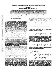
The above equations form a system of five homogeneous equations with unknowns Ex0 , Ey0 , Hx0 , Hy0 , and Hz0 . Because the solutions of the system have to be nontrivial, the determinant of its coefficient matrix should be equal to zero. This leads to:   ω∆t sin =0 (6a) 2     kz ∆z ω∆t µε sin2 sin2 2 2 = (6b) 2 2   ∆z   ∆t   ky ∆y kx ∆x kz ∆z ω∆t sin2 sin2 µε sin2 sin2 2 2 2 2 + + = (6c) ∆x2 ∆y 2 ∆z 2 ∆t2 nπ where kx = mπ a and ky = b . Equation (6a) corresponds to ω = 0. It represents the static solution. Equation (6b) will lead to Hz0 = 0, which does not agree with the assumption of TE modes. Therefore, the remaining (6c) is the numerical dispersion relationship of the TE modes. It is obvious that Equation (6c) is the same as the numerical dispersion relationship of the 3D FDTD method [2] for TEmn mode nπ with kx = mπ a and ky = b . To verify the above claim numerically, we considered a rectangular waveguide where width a = 0.02 m in x direction, height b = 0.01 m in y direction and z was the wave traveling direction. The mesh size was ∆x = 0.001 m, ∆y = 0.001 m, and ∆z = 0.001 m for the 3D FDTD mesh that discretizes the waveguide. The time step size was taken as max ∆t = ∆tmax where ∆tmax is the stability time step limit of the 3D FDTD formulation. TE10 mode was excited with a modulated 2 2 Gaussian pulse sin (2πf0 t) e−(t−t0 ) /T in the center of the structure. Parameter T equaled 20∆t, t0 equaled 60∆t, f0 equaled 60.465 GHz and the corresponding wavelength λg in the waveguide was about

236

Luo and Chen 0.5 Proposed 1D FDTD 0.4

--------- 3D FDTD

0.3

Ey V/m

0.2 0.1 0 -0.1 -0.2 -0.3 -0.4 -0.5

1

1.1

1.2

1.3

1.4

1.5

1.6

1.7

1.8

t (ns)

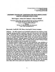
Figure 2. The Ey recorded at a point 300∆z or 60λg away from the source plane. 5∆z = 0.005 m. The recording point was 300∆z or 60λg away from the source plane. Such a long distance between the source and the field recording point allows us to observe effects of the numerical dispersion on the numerical field solutions. Fig. 2 shows the Ey s computed with the 3D FDTD and the proposed 1D FDTD. The difference of the two Ey s computed with the 3D FDTD and the proposed 1D FDTD is shown in Fig. 3. As can be seen, two Ey s overlap almost completely. The maximum difference between the two Ey s is less than 2 × 10−15 (V/m) whereas the maximum field value is around 0.5 (V/m). Such small differences suggest that they are due to computer rounding-off errors. This verifies experimentally the claim we had before: the numerical dispersion relationship of the proposed 1D FDTD is the same as that of the original 3D FDTD. For TM modes, the same conclusion can be reached by following an analysis procedure similar to the one described above. 4. APPLICATIONS OF THE PROPOSED METHOD The proposed method as represented by Equations (2a)–(2f) has two major applications in simulating a waveguide structure: to efficiently generate numerical incident waves (that are required for computing

Progress In Electromagnetics Research, PIER 68, 2007

237

-15

2

x 10

1.5

difference of Ey ( V/m)

1 0.5 0

-0.5 -1

-1.5 -2

1

1.1

1.2

1.3

1.4

1.5

1.6

1.7

1.8

t(n s)

Figure 3. Relative difference between the two Ey s produced by the 1D FDTD and the reference 3D FDTD. electrical parameters such as scattering parameters) and to serve as an efficient wideband absorbing boundary (that is computed only in one dimension). 4.1. Efficient Generation of an Incident Wave Because of its one dimensional nature, the proposed method can be used to obtain an incident wave by computing a long waveguide structure; the waveguide is long enough that the wave reflected by any imperfect termination at the ends can not return to the field recording point and contaminate the incident wave [3]. In the numerical example presented in Section 4, the incident wave obtained with the proposed method is found to be fundamentally the same as that obtained using the conventional 3D FDTD method; the relative differences was less than 10−11 due to the computer rounding-off errors. In other words, the proposed method can produce an incident wave for all intents and purposes identical to that obtained with the conventional 3D FDTD. This results from the fact that the proposed 1D method is derived from the 3D FDTD method and has the same numerical characteristics as that of the 3D FDTD method, as proven before. However, because of its one dimensional nature, the proposed method has much higher computational efficiency than the conventional 3D FDTD method.

238

Luo and Chen

4.2. Absorbing Boundary Condition Since the proposed method can easily simulate a long waveguide structure, it can also be used to terminate a waveguide structure as illustrated in Fig. 4. In it, a waveguide is connected to a discontinuity where both of them are modeled using the conventional 3D FDTD grid. The waveguide is then terminated with the absorbing boundary that is modeled using the proposed 1D FDTD method. Field components Ex |i− 1 , j, k−1 and Ey |i, j− 1 , k−1 are used to pass the field values from the 2 2 3D FDTD grid into the proposed 1D FDTD grid; field components Ey |i, j− 1 , k and Ex |i− 1 , j, k are used to pass the field values in the 2 2 proposed 1D FDTD grid into the 3D FDTD grid.

Figure 4. The proposed absorbing termination using the 1D FDTD mesh. In general, multi-modes exist in the waveguide. However, Equations (2a)–(2f) are valid only for a single mode. To resolve the problem, each mode has to be extracted at the interface between the 3D FDTD mesh and the proposed 1D FDTD mesh. The mode extraction can be performed using the orthogonality of modes as described in [6, 7]. Fig. 5 illustrates such extraction operations. In Fig. 5, each mode corresponds to an independent 1D FDTD mesh line. The positioning of the 1D FDTD mesh lines, i.e., the specific values of i and j in (2a)–(2f), can be the same or can be different for

Progress In Electromagnetics Research, PIER 68, 2007

239

Figure 5. Mode extraction and combination diagram at the interface between the waveguide and the 1D FDTD absorbing termination. the modes. The requirement for the positioning of 1D FDTD mesh line is that it should not be at the null field points of the mode it simulates. In the numerical example presented in Section 5, it is shown that the proposed termination provides an absorption of better than −200 dB in the entire frequency spectrum including the cut-off frequencies. 5. NUMERICAL EXAMPLES We considered the same long waveguide as that used in Section 3: a rectangular waveguide with width a = 0.02 m in x direction, height b = 0.01 m in the y direction and z as the wave propagating direction. The mesh size was ∆x = 0.001 m, ∆y = 0.001 m, and ∆z = 0.001 m. The time step size was taken as ∆t = ∆tmax . The total number of the iterations was 4096 (which amounts to 7.8808 ns of the real time). The source used in the FDTD simulation was the Dirac impulse function δ(n). Matlab was used to program the method and the simulations

240

Luo and Chen

were run on a laptop Pentium-IV PC with 1.8-GHz CPU and 512-MB RAM. The data type used in the simulation is double precision for expected small numbers. For the first application, we computed the incident waves for TE11 mode. The source was placed in the middle of the waveguide. The two ends of the waveguide were terminated with perfect conductors. The field recording points were placed at points 1∆z and 100∆z away from the source plane respectively. The length of the waveguide was 206.8 cm, long enough so that no reflections from the end terminations would reach the field recording points before the 4096 iterations were completed. The structure was then simulated with a reference full-wave 3D FDTD method and the proposed 1D FDTD method; the results for Ey are shown in Figs. 6 and 7 (for clarity, only first 0.5 ns is shown). The maximum relative difference between the Ey obtained with the reference full-wave 3D FDTD simulation and the proposed 1D FDTD simulation is found less than 10−11 , which is invisible in Figs. 6 and 7; it suggests computer-round-off errors as the cause of such a small difference. 0.2

Proposed 1D FDTD

--------- 3D FDTD 0.15

Ey

0.1

0.05

0

-0.05

-0.1

0

0.05

0.1

0.15

0.2

0.25

0.3

0.35

0.4

0.45

0.5

t (ns)

Figure 6. The Ey values of the first 0.5 ns recorded at a point 1∆z away from the source. Table 1 shows the computational expenditures used. As can be seen, the memory used by the proposed 1D method is about 0.6% of that used by the 3D FDTD and CPU time is about 0.23%. The proposed method saves significant amounts of memory and CPU time usage.

Progress In Electromagnetics Research, PIER 68, 2007

241

0.05 0.04

Proposed 1D FDTD

--------- 3D FDTD 0.03 0.02

Ey

0.01 0 -0.01 -0.02 -0.03 -0.04

0

0.05

0.1

0.15

0.2

0.25

0.3

0.35

0.4

0.45

0.5

t (ns)

Figure 7. The Ey values of the first 0.5 ns recorded at a point 100∆z away from the source. Table 1. The memory and CPU time used by the proposed 1D FDTD and the reference 3D FDTD.

Memory CPU time

The reference 3D FDTD 2334 KB 4271 s

The proposed 1D FDTD 14 KB 9.9 s

For the second application, we used the proposed method as the absorbing boundaries to terminate the rectangular waveguides at both ends in order to measure the effectiveness of the absorption. The source was placed 2∆z away from the absorbing boundary placed at the right end of the waveguide and Ey was recorded in between the source and the right absorbing boundary as shown in Fig. 8. Such placements of the source and recording points allowed measurement of the absorption of evanescent modes because they were close to the absorbing boundary. Two cases were simulated. The first was a single-mode case where TE84 was excited. The second case was the multi-mode case where TE10 , TE20 , TE30 , TE40 , TE11 , TE21 , TE31 , TE41 , were

242

Luo and Chen

Figure 8. The positions of the source and the Ey recording point when the 1D FDTD is used as the absorbing boundaries of the 3D FDTD region. excited simultaneously with equal magnitude (the worst case where multiple modes exist). Fig. 9 and Fig. 10 show the computed reflection coefficients in frequency domain. The reflection coefficient was calculated using the following formulae:    E − E ref  y   y |Γ| = 20 log  (7)  (dB)  Eyref  where Eyref is the reference field value computed separately with the conventional 3D FDTD for a very long waveguide. Ey is the field value computed when the proposed 1D FDTD is used as the absorbing boundaries (Fig. 8). It can be seen from Figs. 9 and 10 that the proposed method provides almost perfect absorbing terminating conditions in the entire frequency spectrum from DC to 250 GHz. The reflection coefficients are less then −220 dB even at or below the cut-off frequencies (the cut-off frequencies of TE10 , TE41 and TE84 are 7.5 GHz, 33.54 GHz

Progress In Electromagnetics Research, PIER 68, 2007

243

-240 -250

|Gamma| (dB)

-260 -270 -280 -290 -300 -310 double precision was used

-320

0

50

100

150

200

250

f (GHz)

Figure 9. The computed reflection coefficient for the single-mode case with the proposed 1D FDTD used as the absorbing boundaries shown in Fig. 8. and 84.85 GHz). Such a high absorption indicates the extreme effectiveness of the proposed 1D FDTD absorbing condition. Because both the source and the field recording points are very close to the right absorbing boundary (less than 3∆z away), this means that the proposed method can absorb the evanescent modes very effectively. This is not surprising because the proposed 1D FDTD method has the same numerical dispersion properties as the 3D FDTD method that it connected to. It should be noted that in the above numerical experiments, the numbers of modes excited were chosen arbitrarily to test the performance of the proposed method. In solving a realistic structure, the number of modes to be considered can be decided in the same manner as that employed in the mode matching techniques or in the techniques described in [3–5, 7, 14, 18, 19]. We can also combine the traditional CFS PML method [20, 21] and the proposed 1D FDTD method. The 1D FDTD method is used to absorbing a few most lower order modes which have relatively large values around their cutoff frequencies, the traditional CFS PML can be used to absorbing the remained higher order modes. The hybrid method, which combines the traditional CFS PML method and the proposed 1D FDTD method, is our next step task.

244

Luo and Chen -250 -260

|Gamma| (dB)

-270 -280 -290 -300 -310 -320 double precision was used

-330

0

50

100

150

200

250

f (GHz)

Figure 10. The computed reflection coefficient for the multi-mode case with the proposed 1D FDTD used as the absorbing boundaries shown in Fig. 8. 6. DISCUSSION AND CONCLUSIONS In this paper, a new compact 1D FDTD method for uniformly filled waveguide structures is proposed. It has the same numerical characteristics as the conventional 3D FDTD method. It can be used either to efficiently generate an incident wave or to effectively serve as an almost perfect modal absorbing termination. The differences from the results obtained with the 3D FDTD and the reflection coefficients of the absorbing boundary were found to be extremely small, less than −220 dB in the entire frequency spectrum including the cut-off frequencies, due to the computer rounding-off errors. In other words, the proposed method can handle both propagating and evanescent modes very effectively. In spite of such high effectiveness, the programming of the proposed method is very easy and little analytical pre-processing is required. It should be noted again that the results obtained with the conventional 3D FDTD method were used as the benchmark solutions for comparisons throughout the paper since the conventional method has been proven to be an effective and accurate modeling method.

Progress In Electromagnetics Research, PIER 68, 2007

245

REFERENCES 1. Yee, K. S., “Numerical solution of initial boundary value problems involving Maxwell’s equations in isotropic media,” IEEE Trans. Antennas and Propagations, Vol. 14, No. 3, 302–307, May 1966. 2. Taflove, A. (ed.), Advances in Computational Electrodynamics: the Finite-difference Time-domain Method, Artech House Inc., Norwood, MA, 1998. 3. Huang, T. W., B. Houshmand, and T. Itoh, “Efficient modes extraction and numerically exact matched sources for a homogeneous waveguide cross-section in a FDTD simulation,” IEEE MTT-S International Microwave Symposium Digest, Vol. 1, 31–34, May 1994. 4. Eswarappa, C., P. M. So, and W. J. R. Hoefer, “New procedures for 2-D and 3-D microwave circuit analysis with the TLM method,” IEEE MTT-S International Microwave Symposium Digest, Vol. 2, 661–664, May 1990. 5. Moglie, F., T. Rozzi, P. Marcozzi, and A. Schiavoni, “A new termination condition for the application of FDTD techniques to discontinuity problems in close homogeneous waveguide,” IEEE Microwave and Guided Wave Letters, Vol. 2, No. 12, 475–477, Dec. 1992. 6. Huang, T.-W., B. Houshmand, and T. Itoh, “The implementation of time-domain diakoptics in the FDTD method,” IEEE Transactions on Microwave Theory and Techniques, Vol. 42, No. 11, 2149–2155, Nov. 1994. 7. Righi, M., W. J. R. Hoefer, M. Mongiardo, and R. Sorrentino, “Efficient TLM diakoptics for separable structures,” IEEE Transactions on Microwave Theory and Techniques, Vol. 43, 854– 859, No. 4, Parts 1–2, April 1995. 8. Mrozowski, M., M. Niedzwiecki, and P. Suchomski, “A fast recursive highly dispersive absorbing boundary condition using time domain diakoptics and Laguerre polynomials,” IEEE Microwave and Guided Wave Letters, Vol. 5, No. 6, 183–185, 1995. 9. Mrozowski, M., M. Niedzwiecki, and P. Suchomski, “Improved wideband highly disersive absorbing boundary condition,” Electronics Letters, Vol. 32, No. 12, 1109–1111, June 1996. 10. Alimenti, F., P. Mezzanotte, L. Roselli, and R. Sorrentino, “Modal absorption in the FDTD method: a critical review,” International Journal of Numerical Modeling, Vol. 10, 245–264, 1997. 11. Jung, K. Y., H. Kim, and K. C. Ko, “An improved unimodal absorbing boundary condition for waveguide problems,” IEEE

246

12.

13.

14.

15.

16.

17.

18.

19.

20.

21.

Luo and Chen

Microwave and Guided Wave Letters, Vol. 7, No. 11, 368–370, 1997. Lord, J. A., R. I. Henderson, and B. P. Pirollo, “FDTD analysis of modes in arbitrarily shaped waveguides,” IEE National Conference on Antennas and Propagation, 221–224, March 31– April 1, 1999. Kreczkowski, A., T. Rutkowski, and M. Mrozowski, “Fast modal ABC’s in the Hybrid PEE-FDTD analysis of waveguide discontinuities,” IEEE Microwave and Guided Wave Letters, Vol. 9, No. 5, 186–188, 1999. Alimenti, F., P. Mezzanotte, L. Roselli, and R. Sorrentino, “A revised formulation of modal absorbing and matched modal source boundary conditions for the efficient FDTD analysis of waveguide structures,” IEEE Transactions on Microwave Theory and Techniques, Vol. 48, No. 1, 50–59, Jan. 2000. Luo, S. and Z. Chen, “Efficient one-dimensional FDTD modeling of waveguide structures,” Proceeding of Frontiers in Applied Computational Electromagnetics, 146–149, Victoria, Canada, June 19–20, 2006. Xiao, S., R. Vahldieck, and H. Jin, “Full-wave analysis of guided wave structures using a novel 2-D FDTD,” IEEE Microwave and Guided Wave Letters, Vol. 2, No. 5, 165–167, May 1992. Xiao, S. and R. Vahldieck, “An efficient 2-D FDTD algorithm using real variables,” IEEE Microwave and Guided Wave Letters, Vol. 3, No. 5, 127–129, May 1993. Loh, T. H. and C. Mias, “Implementation of an exact modal absorbing boundary termination condition for the application of the finite-element time-domain technique to discontinuity problems in closed homogeneous waveguides,” IEEE Transactions on Microwave Theory and Techniques, Vol. 52, No. 3, 882–888, Mar. 2004. Lou, Z. and J. M. Jin, “An accurate waveguide port boundary condition for the time-domain finite-element method,” IEEE Transactions on Microwave Theory and Techniques, Vol. 53, No. 9, 3014–3023, Sept. 2005. Kuzuoglu, M. and R. Mittra, “Frequency dependence of the constutive parameters of causal perfectly anisotropic absorbers,” IEEE Microwave and Guided Letters, Vol. 6, 447–449, Dec. 1996. Roden, J. A. and S. D. Gedney, “Convolution PML (CPML): an efficient FDTD implementation of the CFS-PML for arbitrary media,” Microwave and Optical Technology Letters, Vol. 27, No. 5, 334–339, John Wiley and Sons, Dec. 2000.