An efficient P300-based brain-computer interface for disabled subjects Ulrich Hoffmann a,∗,1 , Jean-Marc Vesin a , Touradj Ebrahimi a , Karin Diserens b a Ecole
Polytechnique F´ ed´ erale de Lausanne – Signal Processing Institute, CH–1015 Lausanne – Switzerland Hospitalier Universitaire Vaudois (CHUV), Rue du Bugnon 46, CH–1011 Lausanne – Switzerland
b Centre
Abstract A brain-computer interface (BCI) is a communication system that translates brain-activity into commands for a computer or other devices. In other words, a BCI allows users to act on their environment by using only brain-activity, without using peripheral nerves and muscles. In this paper, we present a BCI that achieves high classification accuracy and high bitrates for both disabled and able-bodied subjects. The system is based on the P300 evoked potential and is tested with five severely disabled and four able-bodied subjects. For four of the disabled subjects classification accuracies of 100% are obtained. The bitrates obtained for the disabled subjects range between 10 and 25 bits/min. The effect of different electrode configurations and machine learning algorithms on classification accuracy is tested. Further factors that are possibly important for obtaining good classification accuracy in P300-based BCI systems for disabled subjects are discussed. Key words: Brain-Computer Interface, P300, Disabled Subjects, Fisher’s Linear Discriminant Analysis, Bayesian Linear Discriminant Analysis
1. Introduction The major goal of BCI research is to develop systems that make it possible for disabled users to communicate with other persons, to control artificial limbs, or to control their environment. To achieve this goal, many aspects of BCI systems are currently being investigated. Research areas include evaluation of invasive and non-invasive technologies to measure brain-activity, development of new BCI applications, evaluation of control-signals (i.e. patterns of brain-activity that can be used for communication), development of algorithms for translation of brain-signals into computer commands, and the development and evaluation of BCI systems specifically for disabled subjects (see Wol∗ Corresponding author. Fax: +41 21 69 37600 E-mail address:
[email protected] 1 U. Hoffmann is supported by Swiss National Science Foundation under Grant No. 200020-112313. Preprint submitted to Elsevier
paw et al. (2002); Lebedev and Nicolelis (2006) for general reviews of BCI research). In this paper, we discuss BCI systems for disabled users based on a noninvasive method to measure brain-activity, namely the electroencephalogram (EEG). One of the earliest systems that used the EEG and was tested with disabled subjects was described by Birbaumer et al. (1999). In their pioneering work, Birbaumer et al. showed that patients suffering from amyotrophic lateral sclerosis (ALS) can use a BCI to control a spelling device and communicate with their environment. The system relied on the fact that patients were able to learn voluntary regulation of slow-cortical potentials, i.e. voltage shifts of the cerebral cortex which occur in the frequency range 1-2 Hz. Drawbacks of the system were that it usually took several months of patient training before the subjects could control the system and that communication was relatively slow. Parallel to the work of Birbaumer et al. BCI 4 March 2007
systems were developed that used changes in brainactivity correlated to motor-imagery as a controlsignal (Pfurtscheller and Neuper, 2001). While these systems were for a long time tested exclusively with able-bodied and quadriplegic subjects, recently tests have been performed with ALS patients and other disabled subjects. Positive results have been obtained by K¨ ubler et al. (2005) who showed that ALS patients can learn to control motor-imagery based BCI systems. However, as for the system based on slow cortical potentials, users were trained over several months and communication was relatively slow. Negative results have been obtained by Hill et al. (2006), who tested a motorimagery based BCI with several completely lockedin patients and could not obtain signals that were suitable for communication. One possible reason for the different results is the fact that in the study of K¨ ubler et al. the patients were not completely locked in whereas the patients in the study of Hill et al. were completely locked in. Furthermore in the study of K¨ ubler et al. several training sessions were used whereas in the work of Hill et al. only one, relatively long training session was used. In summary, it has thus been shown that motor-imagery based systems can be used by disabled subjects, however positive evidence is limited to cases in which subjects were not completely locked-in and followed a long training protocol. In the present work a control-signal is used that can be detected reliably and does not require extended subject training: the P300 event-related potential. The P300 is a positive deflection in the human EEG, appearing approximately 300ms after the presentation of rare or surprising, task-relevant stimuli (Sutton et al., 1965). Farwell and Donchin (1988) were the first to employ the P300 as a controlsignal in a BCI. They described the P300 speller system, with which subjects were able to spell words by sequentially choosing letters from the alphabet. A 6×6 matrix containing the letters of the alphabet and other symbols was displayed on a computer screen. Rows and columns of the matrix were flashed in random order. To choose a symbol, subjects had to silently count how often it was flashed. Flashes of the row or column containing the desired symbol evoked P300-like EEG signals, while flashes of other rows and columns corresponded to neutral EEG signals. The target symbol could be inferred with a simple algorithm that searched for the row and column which evoked the largest P300 amplitude. Since the work of Farwell and Donchin much of
the research in the area of P300 based BCI systems has concentrated on developing new application scenarios (see for example Polikoff et al. (1995); Bayliss (2003)), and on developing new algorithms for the detection of the P300 from possibly noisy data (see for example Xu et al. (2004); Kaper et al. (2004); Rakotomamonjy et al. (2005); Hoffmann et al. (2005); Thulasidas et al. (2006)). Recently, two studies have been published in which P300-based BCI systems were tested with disabled subjects. These studies are described in the following. Piccione et al. (2006) tested a 2D cursor control system with five disabled and seven able-bodied subjects. For cursor control, a four-choice P300 paradigm was used. Subjects had to concentrate on one of four arrows flashing every 2.5 s in random order in the peripheral area of a computer screen. Signals were recorded from one electrooculogram electrode and four EEG electrodes, preprocessed with independent component analysis and classified with a neural network. The results described by Piccione et al. showed that the P300 is a viable control-signal for disabled subjects. However the average communication speed obtained in their study was relatively low when compared to state of the art systems, as for example the systems described by Kaper et al. (2004); Thulasidas et al. (2006). This was the case for the disabled subjects, as well as for able-bodied subjects and can probably be ascribed to the use of signals from only few electrodes, the small number of different stimuli, and long inter stimulus intervals (ISIs). Sellers and Donchin (2006) also used a fourchoice paradigm and tested their system with three subjects suffering from ALS and three able-bodied subjects. In their study four stimuli (’YES’, ’NO’, ’PASS’, ’END’) were presented every 1.4 s in random order, either in the visual modality, in the auditory modality, or in a combined auditory-visual modality. Signals from three electrodes were classified with a stepwise linear discriminant algorithm. The research of Sellers and Donchin showed that P300 based communication is possible for subjects suffering from ALS. The research also showed that communication is possible in the visual, auditory, and combined auditory-visual modality. However, as in the work of Piccione et al., the achieved classification accuracy and communication rate were low when compared to state of the art results. This can again be ascribed to the small number of electrodes, the small number of different stimuli, and long ISIs. In the present work a six-choice P300 paradigm 2
is tested using a population of five disabled and four able-bodied subjects. Six different images were flashed in random order with a stimulus interval of 400 ms. Electrode configurations consisting of four, eight, sixteen and thirty two electrodes were tested. Bayesian Linear Discriminant Analysis (BLDA) and Fisher’s Linear Discriminant Analysis (FLDA) were tested for classification. For four of the disabled subjects and for all the able-bodied subjects communication rates and classification accuracies were obtained that are superior to those of Piccione et al. (2006); Sellers and Donchin (2006). Factors that are possibly important for obtaining good classification accuracy in BCI systems for disabled subjects are discussed. Additionally, to stimulate further research on data analysis techniques for P300-based BCI systems and to enable other researchers to reproduce results, the datasets and some of the algorithms used in the present work are made available for download on the website of the EPFL BCI group (http://bci.epfl.ch/p300). The layout of the paper is as follows. In Section 2 the subject population, the experiments that were performed, and the methods used for data preprocessing and classification are described. Results are given in Section 3. A discussion of the results follows in Section 4. A description of FLDA and BLDA is given in Appendices A and B.
Fig. 1. The display used for evoking the P300. Images were flashed, one at a time, by changing the overall brightness of images.
to digital conversion of the EEG signals. Signal processing and machine learning algorithms were implemented with MATLAB. The stimulus display and the online access to the EEG signals were implemented as dynamic link libraries (DLLs) in C. The DLLs were accessed from MATLAB via a MEX interface. 2.2. Subjects
2. Materials and methods
The system was tested with five disabled and four healthy subjects. The disabled subjects were all wheelchair-bound but had varying communication and limb muscle control abilities (see Table 1). Subjects 1 and 2 were able to perform simple, slow movements with their arms and hands but were unable to control other extremities. Spoken communication with subjects 1 and 2 was possible, although both subjects suffered from mild dysarthria. Subject 3 was able to perform restricted movements with his left hand but was unable to move his arms or other extremities. Spoken communication with subject 3 was impossible. However the patient was able to answer yes/no questions with eye blinks. Subject 4 had very little control over arm and hand movements. Spoken communication was possible with subject 4, although a mild dysarthria existed. Subject 5 was only able to perform extremely slow and relatively uncontrolled movements with hands and arms. Due to a severe hypophony and large
2.1. Experimental setup Users were facing a laptop screen on which six images were displayed (see Fig. 1). The images showed a television, a telephone, a lamp, a door, a window, and a radio. The images were selected according to an application scenario in which users can control electrical appliances via a BCI system. The application scenario served however only as an example and was not pursued in further detail. The images were flashed in random sequences, one image at a time. Each flash of an image lasted for 100 ms and during the following 300 ms none of the images was flashed, i.e. the interstimulus interval was 400 ms. The EEG was recorded at 2048 Hz sampling rate from 32 electrodes placed at the standard positions of the 10-20 international system. A Biosemi Active Two amplifier was used for amplification and analog 3
fluctuations in the level of alertness, communication with subject 5 was very difficult. Subjects 6 to 9 were PhD students recruited from our laboratory (all male, age 30 ± 2.3). None of subjects 6 to 9 had known neurological deficits.
prised on average 810 trials, and the whole data for one subject consisted on average of 3240 trials. 2.4. Offline analysis The impact of different electrode configurations and machine learning algorithms on classification accuracy was tested in an offline procedure. For each subject four-fold cross-validation was used to estimate average classification accuracy. More specifically, the data from three recording sessions were used to train a classifier and the data from the leftout session was used for validation. This procedure was repeated four times so each session served once for validation.
2.3. Experimental schedule Each subject completed four recording sessions. The first two sessions were performed on one day and the last two sessions on another day. For all subjects the time between the first and the last session was less than two weeks. Each of the sessions consisted of six runs, one run for each of the six images. The following protocol was used in each of the runs. (i) Subjects were asked to count silently how often a prescribed image was flashed (For example: ”Now please count how often the image with the television is flashed”). (ii) The six images were displayed on the screen and a warning tone was issued. (iii) Four seconds after the warning tone, a random sequence of flashes was started and the EEG was recorded. The sequence of flashes was block-randomized, this means that after six flashes each image was flashed once, after twelve flashes each image was flashed twice, etc.. The number of blocks was chosen randomly between 20 and 25. On average 22.5 blocks of six flashes were displayed in one run, i.e. one run consisted on average of 22.5 target (P300) trials and 22.5 · 5 = 112.5 non-target (non P300) trials. (iv) In the second, third, and fourth session the target image was inferred from the EEG with a simple classifier 2 . At the end of each run the image inferred by the classification algorithm was flashed five times to give feedback to the user. (v) After each run subjects were asked what their counting result was. This was done in order to monitor performance of the subjects. The duration of one run was approximately one minute and the duration of one session including setup of electrodes and short breaks between runs was approximately 30 minutes. One session com-
2.4.1. Preprocessing Before learning a classification function and before validation, several preprocessing operations were applied to the data. The preprocessing operations were applied in the order stated below. (i) Referencing The average signal from the two mastoid electrodes was used for referencing. (ii) Filtering A 6th order forward-backward Butterworth bandpass filter was used to filter the data. Cutoff frequencies were set to 1.0 Hz and 12.0 Hz. The MATLAB function butter was used to compute the filter coefficients and the function filtfilt was used for filtering. (iii) Downsampling The EEG was downsampled from 2048 Hz to 32 Hz by selecting each 64th sample from the bandpass-filtered data. (iv) Single trial extraction Single trials of duration 1000 ms were extracted from the data. Single trials started at stimulus onset, i.e. at the beginning of the intensification of an image, and ended 1000 ms after stimulus onset. Due to the ISI of 400 ms, the last 600 ms of each trial were overlapping with the first 600 ms of the following trial. (v) Windsorizing Eye blinks, eye movement, muscle activity, or subject movement can cause large amplitude outliers in the EEG. To reduce the effects of such outliers, the data from each electrode were windsorized. For the samples from each electrode the 10th percentile and the 90th percentile were computed. Amplitude values
2
The classifier was trained from the data recorded in the first session. The algorithm described in Hoffmann et al. (2006) was used for preprocessing and the algorithm described in Hoffmann et al. (2004) was used for classification.
4
S1
S2
S3
S4
S5
Diagnosis
Cerebral palsy Multiple sclero- Late-stage Traumatic Post-anoxic sis amyotrophic brain and encephalopathy lateral sclerosis spinal-cord injury, C4 level
Age
56
51
47
33
43
Age at illness onset
0 (perinatal)
37
39
27
37
Sex
M
M
M
F
M
Speech production
Mild disarthria Mild disarthria Severe arthria
Limb muscle control
Weak
Weak
Very weak
Weak
Very weak
Respiration control
Normal
Normal
Weak
Normal
Normal
Normal
Balint’s syndrome
Voluntary eye move- Normal ment
Mild mus
nystag- Normal
dis- Mild disarthria Severe hypophony
Table 1 Subjects from which data was recorded in the study of the environment control system.
lying below the 10th percentile or above the 90th percentile were then replaced by the 10th percentile or the 90th percentile, respectively. (vi) Scaling The samples from each electrode were scaled to the interval [−1, 1]. (vii) Electrode selection Four electrode configurations with different numbers of electrodes were tested. The electrode configurations are shown in Fig. 2. (viii) Feature vector construction The samples from the selected electrodes were concatenated into feature vectors. The dimensionality of the feature vectors was Ne × Nt , where Ne denotes the number of electrodes and Nt denotes the number of temporal samples in one trial. Due to the trial duration of 1000 ms and the downsampling to 32 Hz, Nt always equalled 32. Depending on the electrode configuration Ne equalled 4, 8, 16, or 32.
sions and validated on the left-out fourth session. Training data sets contained 405 target trials and 2025 non-target trials and validation data sets consisted of 135 target and 675 non-target trials (these are average values cf. Section 2.3). Bayesian Linear Discriminant Analysis (BLDA) was used to learn classifiers (see Appendix B). To compare the performance of BLDA with a standard algorithm, in a second set of experiments classifiers were computed with Fisher’s Linear Discriminant Analysis (FLDA) (see Appendix A). Both algorithms were fully automatic, i.e. no user intervention was required to adjust hyperparameters, and the computation of classifiers took less than one minute on a standard PC. After the classifiers had been trained, they were applied to validation data in the following way. For each run in the validation session, the single trials corresponding to the first twenty blocks of flashes were extracted using the preprocessing operations. Then the single trials were classified. This resulted in twenty blocks of classifier outputs. Each block consisted of six classifier outputs, one output for each image on the display. To decide which image the user was concentrating on, the classifier outputs were summed over blocks for each image and
2.4.2. Machine learning and classification Classifiers and the percentile values used for windsorizing were trained on the data from three ses5
Fp1
Fp2
AF3 Fz
Fz
Cz
Cz
FC1 C3
P7
P3
Pz
P4
P8
P7
P3
C4
T7
CP2 Pz
F3
FC5
FC2 Cz
CP1 Pz
F7
Fz
P4
FC1 C3
P7
CP1 P3
O1
Oz
Oz
O2
C4 CP2
Pz
O1
F8 FC6
FC2
PO3 Oz
F4
Cz
CP5 P8
AF4 Fz
P4
T8 CP6 P8
PO4 Oz
O2
Fig. 2. Electrode configurations used in the experiments. From left to right: Configuration I (4 electrodes), configuration II (8 electrodes), configuration III (16 electrodes), and configuration IV (32 electrodes).
then the image with the maximum summed classifier output was selected. Different tradeoffs between the time needed to take a decision and the classification accuracy were simulated by varying the number of summed classifier outputs, i.e. the number of blocks.
after 12 or more blocks of stimulus presentations were averaged (i.e. after 28.8 s). Subject 6 reported that he accidentally concentrated on the wrong stimulus during one run in session 1. This explains the lower average classification accuracy for this subject. In all other runs the average classification accuracy after more than 12 blocks was 100% for subject 6. The somewhat lower performance for subject 9 is restricted to session 4, i.e. in sessions 1 to 3 subject 9 always reached 100% classification accuracy. The reason for the lower performance in session 4 might be fatigue. The best performance was achieved by subject 8. Subject 8 was highly concentrated and motivated during the experiments. It is known that motivation and arousal in general increase P300 amplitude (Carrillo-de-la Pena and Cadaveira, 2000). One possible explanation for the very good performance of subject 8 might thus be the fact that the subject was very motivated.
3. Results 3.1. General observations In Fig. 3 classification accuracy averaged over sessions and the corresponding bitrates are plotted against the time needed to take a decision. Electrode configuration (II) in conjunction with BLDA as classification method was used for the graphs in Fig. 3 3 and the bitrates were computed by applying the definition of Wolpaw et al. (2002) to the average accuracy curves. The bitrates for all possible combinations of electrode configuration and classification algorithm are listed in Table 2. Data for subject 5 are not included in Fig. 3 and in Table 2 because classification accuracies above chance level could not be obtained. During the experiments a speech therapist helped to communicate with subject 5. However it was not clear if the subject understood the instructions given before the experiments. Furthermore the level of alertness of the subject fluctuated strongly and rapidly during experiments. All of the subjects, except for subjects 6 and 9, achieved an average classification accuracy of 100%
3.2. Differences between disabled and able-bodied subjects The differences that can be observed between disabled and able-bodied subjects depend on the performance measure used. If maximum classification accuracy is used as performance measure no differences can be found between able-bodied and disabled subjects. This is shown for classification with BLDA and the eight electrodes configuration in Fig. 3. The same behavior was found for the other combinations of classifier and electrode configuration (not shown). If bitrate is used as performance measure, differences between disabled and able-bodied subjects can readily be observed. Able-bodied subjects achieved higher maximum bitrates than disabled subjects. This was the case for
3
Electrode configuration (II) was chosen for plotting because it represents a good tradeoff between classification performance and practical applicability of a BCI system. To keep the plots uncluttered, the curves for FLDA, which for electrode configuration (II) are very similar to those of BLDA, are not shown.
6
45
80
40
70
35
60
30
50
25
40
20
S1
30
Accuracy (%)
20
S2
S3
S4
15 10
10
5
0
0
100
50
90
45
80
40
70
35
60
30
50
25
40
20
S6
30 20
S7
S8
S9
10 0 0
Bitrate (bits/min)
0
90
15
Bitrate (bits/min)
Accuracy (%)
100
10 5
5
10
15
20 25 30 Time (s)
35
40
45
50
0
5
10
15
20 25 30 Time (s)
35
40
45
50
0
5
10
15
20 25 30 Time (s)
35
40
45
50
0
5
10
15
20 25 30 Time (s)
35
40
45
0 50
Fig. 3. Classification accuracy and bitrate plotted vs. time. The panels show the classification accuracy obtained with BLDA and the eight electrode configuration, averaged over four sessions (circles) and the corresponding bitrate (crosses), for disabled subjects (S1-S4) and able-bodied subjects (S6-S9).
all combinations of classifier and electrode configuration (see Table 2). Closely linked to maximum bitrate is the classification accuracy for small numbers of blocks of presentations. For this measure of performance, differences between able-bodied and disabled subjects can also be observed. The classification accuracy of disabled subjects (especially of subjects 1 and 2) increases more slowly than that of the able-bodied subjects (see Fig. 3).
100
Accuracy (%)
90
80
70 32 electrodes 16 electrodes 8 electrodes 4 electrodes
60
50 0
3.3. Electrode configurations and classification methods
5
10
15
20 25 30 Time (s)
35
40
45
50
Fig. 4. Classification accuracy obtained with BLDA, averaged over all subjects and sessions, plotted against time, for all electrode configurations.
Using different electrode configurations in conjunction with BLDA yielded the performance curves shown in Fig. 4. The performance curves obtained with FLDA are shown in Fig. 5. For both figures, classification accuracy was averaged over sessions and over all subjects. For both classification methods a strong increase in classification accuracy can be observed between the electrode configurations consisting of four and eight electrodes. Using more than eight electrodes yielded only relatively small increases in performance for BLDA and resulted in a decrease of performance for FLDA (cf. Figs. 4, 5, Table 2). For the configurations consisting of four and eight electrodes, the classification accuracy and bitrates obtained with BLDA were slightly better than those obtained with FLDA. For the configurations consisting of more than eight electrodes the performance of BLDA was clearly better than that
of FLDA. For all electrode configurations the differences in accuracy between BLDA and FLDA were strongest when only a small number of blocks was used, i.e. in the range 0–20 s. (cf. Figs. 4, 5). 3.4. Averaged waveforms Detecting the target image from a sequence of EEG trials relies on differences between the waveforms of target and non-target trials. To visualize these differences the averaged waveforms at electrode Pz are plotted in Fig. 6 4 . As expected, disabled subjects and able-bodied subjects show a 4
Electrode Pz was chosen for plotting because it typically shows the largest P300 amplitude.
7
Subject
BLDA-4 BLDA-8 BLDA-16 BLDA-32 FLDA-4
FLDA-8 FLDA-16 FLDA-32
S1
8.8
8.8
7.7
13.0
6.2
7.1
5.0
6.5
S2
6.8
10.8
11.4
11.2
6.8
13.0
6.3
6.3
S3
21.9
24.7
24.7
21.9
24.7
28.0
28.0
19.3
S4
14.9
19.3
21.9
29.8
13.1
17.0
19.0
14.9
S6
25.9
25.9
25.9
34.1
22.3
22.3
17.0
13.1
S7
22.3
22.3
38.7
38.7
19.0
19.3
21.9
19.3
S8
38.7
49.4
56.0
64.6
43.8
56.3
49.9
38.7
S9
17.0
19.3
22.3
17.0
8.0
13.0
14.9
13.0
Avg. (S1-S4) 13.1±6.8 15.9±7.5 16.4±8.2 19.0±8.6 12.7±8.6 16.3±8.8 14.6±11.0 11.7±6.5 Avg. (S6-S9) 26.0±9.2 29.3±13.7 35.7±15.2 38.6±19.7 23.3±15.0 27.6±19.3 25.8±16.0 21.0±12.1 Avg. (All) 19.5±10.2 22.6±12.5 26.1±15.3 28.8±17.6 18.0±12.6 22.0±15.2 20.2±14.1 16.4±10.3 Table 2 Maximum average bitrate per minute. Bitrates were computed from average accuracy curves and are shown for all combinations of classification algorithm and electrode configuration. Mean bitrate and standard deviations were computed for disabled subjects (S1-S4), able bodied subjects (S6-S9), and all subjects. 3
100
Amplitude (uV)
2
80
1 0 −1 −2
70
−3
50 0
3
32 electrodes 16 electrodes 8 electrodes 4 electrodes
60
5
10
15
20 25 30 Time (s)
35
40
45
2 Amplitude (uV)
Accuracy (%)
90
50
Fig. 5. Classification accuracy obtained with FLDA, averaged over all subjects and sessions, plotted against time, for all electrode configurations.
1 0 −1 −2 −3 0
P300-like peak in the target condition which is not present in the non-target condition. The latency of the P300 is higher for the disabled subjects (around 500 ms) when compared to the one from ablebodied subjects (around 300 ms). The amplitude at the P300 peak is smaller for the disabled subjects (around 1.5 µV) than for the able-bodied subjects (around 2 µV).
100
200
300
400 500 Time (ms)
600
700
800
Fig. 6. Top: Average waveforms at electrode Pz for disabled subjects (S1-S4). Bottom: Average waveforms at electrode Pz for able-bodied subjects (S6-S9). Shown are the average responses to target stimuli (solid line) and non-target stimuli (dashed line) from all four sessions. A prestimulus interval of 100 ms was used for baseline correction of single trials.
high. In the work of Sellers and Donchin (2006) the best classification accuracy for the able-bodied subjects was on average 85% and the best classification accuracy for the ALS patients was on average 72% (values taken from Table 3 in Sellers and Donchin (2006)). In the present study the best classification accuracy for the able-bodied subjects was on average close to 100% and the best classification accuracy for disabled subjects was on average 100% (see Fig. 3). Bitrates in bits/min were not reported in the study
4. Discussion 4.1. Differences to other studies Compared to other P300-based BCI systems for disabled users, the classification accuracy and bitrate obtained in the current study are relatively 8
of Sellers and Donchin. In the work of Piccione et al. (2006) average bitrates of about 8 bits/min were reported for both disabled and able-bodied subjects. In the present study the average bitrate obtained with electrode configuration (II) was 15.9 bits/min for the disabled subjects and 29.3 bits/min for the able-bodied subjects. Due to differences in experimental paradigms and subject populations the classification accuracy and bitrate obtained in the two studies described above cannot be compared directly to those obtained in the present study. Nevertheless, several factors that might have caused the differences can be identified. These factors are described below.
culties to stay concentrated during long runs and thus P300 amplitude and classification accuracy might actually decrease for longer ISIs. Regarding bitrate, the factors described above have to be considered together with the fact that for a given classification accuracy higher bitrates are obtained with shorter ISIs. Additionally one has to consider that if the ISI is made too short, subjects with cognitive deficits might have problems to detect all target stimuli and classification accuracy might decrease. Given the complex interrelationship of several factors an optimal ISI for P300-based BCIs can only be determined experimentally. Here we have shown that an ISI of 400 ms yields good results. Sellers and Donchin have used an ISI of 1.4 s, and Piccione et al. have used an ISI of 2.5 s. The results obtained in their studies seem to indicate that these ISIs are too long.
– Number of choices In the present study a six-choice paradigm was used, whereas in the experiments of Sellers and Donchin and Piccione et al. four-choice paradigms were used. As a consequence the target stimulus occurred with a probability of 0.25 in the experiments of Sellers and Donchin and Piccione et al., whereas in the present work it occurred with a probability of 0.16. Smaller target probabilities correspond to higher P300 amplitudes (DuncanJohnson and Donchin, 1977), thus the P300 in our system might have been easier to detect. In general, when designing a P300-based BCI, one has to take into account that disabled subjects might suffer from visual impairments. Systems such as the P300 speller in which users have to focus on a relatively small area of the display might thus not be appropriate for disabled subjects. Reducing the number of choices enlarges the area occupied by one item on the screen and thus facilitates concentration on one item. This might be particularly important for subjects who have little remaining control over their eyemovements. Such subjects might use covert shifts of visual attention (Posner and Petersen, 1990) to control a P300-based BCI, which should be easier when a small number of large items is used.
4.2. Electrode configurations The electrode configuration used in a BCI determines the suitability of the system for daily use. Clearly, systems that use only few electrodes take less time for setup and are more user friendly than systems with many electrodes. However, if too few electrodes are used not all features that are necessary for accurate classification can be captured and communication speed decreases. For P300-based BCI systems different electrode configurations have been described in the literature. Good results have been reported using only three or four midline electrodes (Fz, Cz, Pz, Oz) (Serby et al., 2005; Sellers and Donchin, 2006; Piccione et al., 2006). Krusienski et al. (2006) described an eight electrode configuration consisting of the midline electrodes and the four parietal-occipital electrodes PO7, PO8, P3, and P4. Kaper et al. (2004) employed a ten electrode configuration consisting of the midline electrodes, the parietal-occipital electrodes PO7, P08, P3, P4 and the central electrodes C3, C4. Thulasidas et al. (2006) used a set of 25 central and parietal electrodes. Here we have tested different electrode configurations, consisting of 4, 8, 16, and 32 electrodes, in combination with the BLDA and FLDA classification algorithms. The results show that for both algorithms a significant increase in classification accuracy can be obtained by augmenting the set of four midline electrodes with the parietal electrodes
– Interstimulus interval Several factors have to be kept in mind when choosing an ISI for a P300-based BCI system. Regarding classification accuracy, longer ISIs theoretically yield better results. This should be the case because longer ISIs (within some limits) cause larger P300 amplitude. On the other hand, a consequence of long ISIs is a longer overall duration of runs. Disabled subjects might have diffi9
P7, P3, P4, and P8. For most of the subjects, inspection of the average waveforms at the parietal electrodes showed that in target trials there was a negative peak with a latency of about 200 ms which was weaker in the non-target condition. This N200like component probably is responsible for the increase of classification accuracy when the parietal electrodes are included. Further research is needed to clarify the possible functional significance of this component. With the BLDA algorithm a small further increase in classification accuracy could be obtained by using the configurations consisting of 16 or 32 electrodes. With the FLDA algorithm, classification decreased when more than 8 electrodes were used. This probably happened because the FLDA algorithm is unable to deal with training data sets in which the number of features is large compared to the number of training examples. In summary, regardless of the classification algorithm that is used, the eight electrode configuration represents a good compromise between suitability for daily use and classification accuracy and seems to capture most of the important features for P300 classification.
scatter matrix (see Appendix A). This allows to use FLDA, even if the number of features is high. However, with this approach the performance of FLDA deteriorated when the number of electrodes was increased. In BLDA, the small sample size problem, and more generally the problem of overfitting are solved by using regularization. Through a Bayesian analysis, the degree of regularization can be automatically estimated from training data without the need for user intervention or time consuming cross-validation (see Appendix B). With the datasets used in this work, the BLDA algorithm is superior to FLDA in terms of classification accuracy and bitrates, especially if the number of features is large. A further advantage, which was however not exploited in this work, is that the BLDA algorithm yields probabilistic outputs. In summary, BLDA is an interesting alternative to FLDA which offers good classification accuracy and does not constrain the practical applicability of a BCI system.
4.3. Machine learning algorithms
In this work an efficient P300-based BCI system for disabled subjects was presented. We have shown that high classification accuracies and bitrates can be obtained for severely disabled subjects. Due to the use of the P300, only a small amount of training was required to achieve good classification accuracy. Future improvements to the work presented here might consist in testing the system with completely locked-in patients and in defining useful BCI applications adapted to the needs of disabled users. Also it might be useful to perform studies with larger numbers of subjects in order to confirm the results found in the present work.
5. Conclusion
Many of the characteristics of a BCI system depend critically on the employed machine learning algorithm. Important characteristics that are influenced by the machine learning algorithm are classification accuracy and communication speed, as well as the amount of time and user intervention necessary for setting up a classifier from training data. A simple and efficient algorithm that has relatively often been used in P300-based and other BCI systems is FLDA (Pfurtscheller and Neuper, 2001; Bostanov, 2004; Kaper, 2006). In a comparison of classification techniques (Krusienski et al., 2006) for P300-based BCIs, FLDA was among the best methods in terms of classification accuracy and ease of use. However, using FLDA becomes impossible when the number of features becomes large, relative to the number of training examples. This is known as the small sample size problem. The small sample size problem occurs because the between-class scatter matrix used in FLDA becomes singular when the number of features becomes large. In the present study the solution to this problem was to use the Moore-Penrose pseudoinverse of the between-class
Acknowledgements Many thanks go to all the subjects who volunteered to participate in the experiments described in this paper. We would also like to Viviane Chevalley for perfect organization of the EEG recording sessions. Finally we would like to thank Michael Ansorge, Johannes Hoffmann, Yannick Maret, and David Marimon for proofreading the manuscript. 10
Appendix A. Fisher’s LDA (FLDA)
larger than the number of training examples N . A simple solution for this problem is to replace the in† verse S−1 W by the Moore-Penrose pseudo-inverse SW (Tian et al., 1988). The optimal solution for w then reads:
The goal in Fisher’s linear discriminant analysis (FLDA) is to compute a discriminant vector that separates two or more classes as well as possible. Here we consider only the two-class case. We are given a set of input vectors xi ∈ RD , i ∈ {1 . . . N } and corresponding class-labels yi ∈ {−1, 1}. Denoting by N1 the number of training examples for which yi = 1, by C1 the set of indices i for which yi = 1, and using analogous definitions for N2 , C2 , the objective function for computing a discriminant vector w ∈ RD is (µ1 − µ2 )2 J(w) = , (A.1) σ12 + σ22 where X 1 X T µk = w xi , σk2 = (wT xi − µk )2 . Nk i∈Ck
w ∝ S†W (m1 − m2 ).
The output of FLDA given an input vector x ˆ is simply the product wT x ˆ. In the P300-based BCI described in the present study, the output of FLDA was summed over trials and the image corresponding to the maximum of the summed output values was then selected (cf. Section 2.4.2).
Appendix B. Bayesian LDA (BLDA) BLDA can be seen as an extension of Fisher’s Linear Discriminant Analysis (FLDA). In contrast to FLDA, in BLDA regularization is used to prevent overfitting to high dimensional and possibly noisy datasets. Through a Bayesian analysis the degree of regularization can be estimated automatically and quickly from training data without the need for time consuming cross-validation. We have obtained very good results with BLDA and we think that the BLDA algorithm might be of general interest to the BCI community. A MATLAB implementation of BLDA can be downloaded from the webpage of the EPFL BCI group (http://bci.epfl.ch/p300). Algorithms that are closely related to the method presented below are the Bayesian least-squares support vector machine (Van Gestel et al., 2002) and the algorithm for Bayesian non-linear discriminant analysis described by Centeno and Lawrence (2006). BLDA is also closely related to the so-called evidence framework for which detailed accounts are given by MacKay (1992); Bishop (2006). As a starting point for the description of BLDA we use the fact that FLDA is a special case of least squares regression. Least squares regression is equivalent to FLDA if regression targets are set to NN1 for examples from class 1 and to − NN2 for examples from class -1 (where N is the total number of training examples, N1 the number of examples from class 1, and N2 the number of examples from class -1). A proof for the equivalence between least squares regression and FLDA can be found in the book of Bishop (2006). Given the connection between regression and FLDA, our approach for BLDA is to
i∈Ck
(A.2) This means that one is searching for discriminant vectors that result in a large distance between the projected means and small variance around the projected means (small within-class variance). To compute directly the optimal discriminant vector for a training data set, matrix equations for the quantities (µ1 − µ2 )2 and σ12 + σ22 can be used. We first define the class means mk . 1 X mk = xi (A.3) Nk i∈Ck
Now we can define the between-class scatter matrix SB and the within-class scatter matrix SW . SB =(m1 − m2 )(m1 − m2 )T SW =
2 X X
(xi − mk )(xi − mk )T
(A.4) (A.5)
k=1 i∈Ck
With the help of these two matrices the objective function for FLDA can be written as a Rayleigh quotient. wT SB w J(w) = T (A.6) w SW w By computing the derivative of J and setting it to zero, one can show that the optimal solution for w satisfies the following equation: w ∝ S−1 W (m1 − m2 ).
(A.8)
(A.7)
A potential problem in FLDA is that the betweenclass scatter matrix can become singular, and the inverse of SW can become ill-defined. In particular this happens when the number of features D becomes 11
perform regression in a Bayesian framework and set target values as mentioned above. The assumption in Bayesian regression is that targets t and feature vectors x are linearly related with additive white Gaussian noise n.
Since both prior and likelihood are Gaussian, the posterior is also Gaussian and its parameters can be derived from likelihood and prior by completing the square. The mean m and covariance C of the posterior satisfy the following equations.
t = wT x + n
m = β(βXXT + I0 (α))−1 Xt
(B.6)
C = (βXXT + I0 (α))−1
(B.7)
(B.1)
Given this assumption, we can write down the likelihood function for the weights w used in regression: µ ¶ N2 β β p(D|β, w) = exp(− kXT w − tk2 ). (B.2) 2π 2 Here t denotes a vector containing the regression targets, X denotes the matrix that is obtained from the horizontal stacking of the training feature vectors, D denotes the pair {X, t}, β denotes the inverse variance of the noise, and N denotes the number of examples in the training set. It is assumed that the feature vectors contain one feature which always equals one; the bias term which is commonly used in regression can thus be omitted. To perform inference in a Bayesian setting we have to specify a prior distribution for the latent variables, i.e. for the weight vector w. The expression for the prior distribution is: ³ α ´ D2 ³ ² ´ 12 1 p(w|α) = exp(− wT I0 (α)w), 2π 2π 2 (B.3) where I0 (α) is a square, D + 1 dimensional, diagonal matrix α 0 ... 0 0 α . . . 0 0 I (α) = . . . . (B.4) , .. .. . . ..
By multiplying the likelihood function (equation B.2) for a new input vector x ˆ with the posterior distribution (equation B.5) followed by an integration over w, we obtain the predictive distribution, i.e. the probability distribution over regression targets conditioned on an input vector: Z p(tˆ|β, α, x ˆ, D) = p(tˆ|β, x ˆ, w)p(w|β, α, D) dw. (B.8) The predictive distribution is again Gaussian and can be characterized by its mean µ and its variance σ2 . µ = mT x ˆ 1 2 σ = +x ˆT Cˆ x β
(B.9) (B.10)
In the P300-based BCI described in the present study, only the mean value of the predictive distribution was used for taking decisions. More precisely, mean values were summed over trials and the image corresponding to the maximum of the summed mean values was then selected (cf. Section 2.4.2). In a more general setting, class probabilities could be obtained by computing the probability of the target values used during training. Using the predictive distribution from equation B.8 and omitting the conditioning on β, α, D we could use:
0 0 ... ² and D is the number of features. The prior for the weights thus is an isotropic, zero-mean Gaussian distribution. The effect of using a zero-mean Gaussian prior for the weights is similar to the effect of the regularization term used in ridge regression and regularized FLDA. The estimates for w are shrunk towards the origin and the danger of overfitting is reduced. The prior for the bias (the last entry in w) is a zero-mean univariate Gaussian. Setting ² to a very small value, the prior for the bias is practically flat. This expresses the fact that a priori we do not make assumptions about the value of the bias parameter. Given likelihood and prior the posterior distribution can be computed using Bayes rule. p(D|β, w)p(w|α) . (B.5) p(w|β, α, D) = R p(D|β, w)p(w|α) dw
p(ˆ y = 1|ˆ x) =
p(tˆ = p(tˆ =
N1 x) N |ˆ
N1 x) N |ˆ
+ p(tˆ =
−N2 x) N |ˆ
.
(B.11) Both the posterior distribution and the predictive distribution depend on the hyperparameters α and β. We have assumed above that the hyperparameters are known, however in real-world situations the hyperparameters are usually unknown. One possibility to solve this problem would be to use crossvalidation to determine the hyperparameters that yield the best prediction performance. However, the Bayesian regression framework offers a more elegant and less time-consuming solution for the problem of choosing the hyperparameters. The idea is to write down the likelihood function for the hyperparameters and then maximize the likelihood with respect 12
to the hyperparameters. The maximum likelihood solution for the hyperparameters can be found with a simple iterative algorithm which we do not discuss in detail here but which is described by MacKay (1992); Bishop (2006).
Ebrahimi, T., 2004. Application of the evidence framework to brain-computer interfaces. In: Proceedings of the IEEE Engineering in Medicine and Biology Conference. Hoffmann, U., Vesin, J.-M., Ebrahimi, T., 2006. Spatial filters for the classification of event-related potentials. In: Proceedings of the 14th European Symposium on Artificial Neural Networks (ESANN). Kaper, M., 2006. P300-based brain-computer interfacing. Ph.D. thesis, University of Bielefeld, Germany. Kaper, M., Meinicke, P., Grosskathoefer, U., Lingner, T., Ritter, H., 2004. Support vector machines for the P300 speller paradigm. IEEE Trans. Biomed. Eng. 51 (6), 1073–1076. Krusienski, D. J., Sellers, E. W., Cabestaing, F., Bayoudh, S., McFarland, D. J., Vaughan, T. M., Wolpaw, J. R., 2006. A comparison of classification techniques for the P300 speller. J. Neur. Eng. 3 (4), 299–305. K¨ ubler, A., Nijboer, F., Mellinger, J., Vaughan, T., Pawelzik, H., Schalk, G., McFarland, D., Birbaumer, N., Wolpaw, J., 2005. Patients with ALS can use sensorimotor rhythms to operate a braincomputer interface. Neurology 64, 1775–1777. Lebedev, M. A., Nicolelis, M. A., 2006. Brainmachine interfaces: past, present and future. Trends in Neurosciences 29 (9), 536–546. MacKay, D. J. C., 1992. Bayesian interpolation. Neural Comput. 4 (3), 415–447. Pfurtscheller, G., Neuper, C., 2001. Motor imagery and direct brain-computer communication. Proceedings of the IEEE 89 (7), 1123–1134. Piccione, F., Giorgi, F., Tonin, P., Priftis, K., Giove, S., Silvoni, S., Palmas, G., Beverina, F., 2006. P300-based brain-computer interface: Reliability and performance in healthy and paralysed participants. Clin. Neurophysiol. 117 (3), 531–537. Polikoff, J., Bunnell, H., Borkowski, W., 1995. Toward a P300-based computer interface. In: Proceedings of the RESNA ’95 Annual Conference. Posner, M. I., Petersen, S. E., 1990. The attention system of the human brain. Annual Review of Neuroscience 13 (1), 25–42. Rakotomamonjy, A., Guigue, V., Mallet, G., Alvarado, V., 2005. Ensemble of SVMs for improving brain-computer interface P300 speller performances. In: Proceedings of International Conference on Neural Networks (ICANN). Sellers, E., Donchin, E., 2006. A P300-based braincomputer interface: Initial tests by ALS patients.
References Bayliss, J. D., 2003. Use of the evoked P3 component for control in a virtual apartment. IEEE Trans. Neural Syst. Rehab. Eng. 11 (2), 113–116. Birbaumer, N., Hinterberger, T., Iversen, I., Kotchoubey, B., K¨ ubler, A., Perelmouter, J., Taub, E., Flor, H., 1999. A spelling device for the paralysed. Nature 398, 297–298. Bishop, C. M., 2006. Pattern Recognition and Machine Learning. Springer. Bostanov, V., 2004. Feature extraction from eventrelated brain potentials with the continuous wavelet transform and the t-value scalogram. IEEE Trans. Biomed. Eng. 51 (6), 1057–1061. Carrillo-de-la Pena, M. T., Cadaveira, F., 2000. The effect of motivational instructions on P300 amplitude. Neurophysiologie Clinique/Clinical Neurophysiology 30 (4), 232–239. Centeno, T., Lawrence, N., 2006. Optimising kernel parameters and regularisation coefficients for nonlinear discriminant analysis. Journal of Machine Learning Research 7, 455–491. Duncan-Johnson, C., Donchin, E., 1977. On quantifying surprise. The variation of event related potentials with subjective probability. Psychophysiology 14 (5), 456–467. Farwell, L. A., Donchin, E., 1988. Talking off the top of your head: toward a mental prosthesis utilizing event-related brain potentials. Electroencephalogr. Clin. Neurophysiol. 70, 510–523. Hill, N., Lal, T., Schr¨oder, M., Hinterberger, T., Wilhelm, B., Nijboer, F., Mochty, U., Widman, G., Elger, C., Sch¨olkopf, B., K¨ ubler, A., Birbaumer, N., 2006. Classifying EEG and ECoG signals without subject training for fast BCI implementation: Comparison of nonparalyzed and completely paralyzed subjects. IEEE Trans. Neural Syst. Rehab. Eng. 14 (2), 183–186. Hoffmann, U., Garcia, G. N., Diserens, K., Vesin, J.-M., Ebrahimi, T., 2005. A boosting approach to P300 detection with application to braincomputer interfaces. In: Proceedings of the IEEE EMBS Neural Engineering Conference. Hoffmann, U., Garcia, G. N., Vesin, J.-M., 13
Clin. Neurophysiol. 117 (3), 538–548. Serby, H., Yom-Tov, E., Inbar, G., 2005. An improved P300-based brain-computer interface. IEEE Trans. Neural Syst. Rehab. Eng. 13 (1), 89– 98. Sutton, S., Braren, M., Zubin, J., John, E., 1965. Evoked-potential correlates of stimulus uncertainty. Science 150 (700), 1187–1188. Thulasidas, M., Guan, C., Wu, J., 2006. Robust classification of EEG signal for brain-computer interface. IEEE Trans. Neural Syst. Rehab. Eng. 14 (1), 24–29. Tian, Q., Fainman, Y., Lee, S. H., 1988. Comparison of statistical pattern-recognition algorithms for hybrid processing. II. Eigenvector-based algorithm. J. Opt. Soc. Am. A 5, 1670–1682. Van Gestel, T., Suykens, J., Lanckriet, G., Lambrechts, A., De Moor, B., Vandewalle, J., 2002. Bayesian framework for least-squares support vector machine classifiers, gaussian processes, and kernel fisher discriminant analysis. Neural Computation 14 (5), 1115–1147. Wolpaw, J. R., Birbaumer, N., McFarland, D. J., Pfurtscheller, G., Vaughan, T. M., June 2002. Brain-computer interfaces for communication and control. Clin. Neurophysiol. 113 (6), 767–791. Xu, N., Gao, X., Hong, B., Miao, X., Gao, S., Yang, F., 2004. BCI competition 2003 Data Set IIb: Enhancing P300 wave detection using ICA-based subspace projections for BCI applications. IEEE Trans. Biomed. Eng. 51 (6), 1067–1072.
14