an efficient proactive reactive scheduling approach to ... - LAMSADE

AN EFFICIENT PROACTIVE REACTIVE SCHEDULING APPROACH TO HEDGE AGAINST SHOP FLOOR DISTURBANCES Mohamed Ali Aloulou Laboratoire d’Informatique de Paris 6 8, rue du Capitaine Scott 75015 Paris, France [email protected]

Marie-Claude Portmann MACSI team of INRIA-Lorraine and LORIA-UHP-INPL Ecole des Mines de Nancy Parc de Saurupt, 54042 Nancy Cedex, France [email protected]

Abstract

We consider the single machine scheduling problem with dynamic job arrival and total weighted tardiness and makespan as objective functions. The machine is subject to disruptions related to late raw material arrival and machine breakdowns. We propose a proactive-reactive approach to deal with possible perturbations. In the proactive phase, instead of providing only one schedule to the decision maker, we present a set of predictive schedules. This set is characterized by a partial order of jobs and a type of associated schedules, here semi-active schedules. This allows to dispose of some flexibility in job sequencing and flexibility in time that can be used on-line by the reactive algorithm to hedge against unforeseen disruptions. We conduct computational experiments which prove that our approach outperforms a predictive reactive approach particularly for disruptions with low to medium amplitude.

Keywords: scheduling, single machine, flexibility, robustness, total weighted tardiness, genetic algorithms.

1

2

1.

Introduction

Scheduling is an important element of production systems because it allows improving the performance of the system and serves as an overall plan on which many other shop activities are based. Several techniques have been proposed to generate, for a given problem, a unique schedule satisfying the shop constraints and providing optimal or near optimal performance. However, when this pre-computed or predictive schedule is released for execution, continual adapting is required to take into account the presence of uncertainties. These uncertainties are related for example to machine breakdowns, staffing problems, unexpected arrival of new orders, early or late arrival of raw material and uncertainties in the duration of processing times [9]. When the first perturbations arise, the schedule is slightly modified and the performance is a little bit affected. But when there are more important perturbations, the performance of the final schedule becomes generally much worse than the initial one. Besides, the predictive schedule is also used as a basis for planning activities, such as raw material procurement, preventive maintenance and delivery of orders to external or internal customers [16]. Consequently, if the obtained schedule deviates considerably from the initial predictive schedule, then this may delay the execution of many activities related to internal customers. It may also add some costs due to early procurement of raw material from suppliers or late delivery of finished products to external customers. Therefore, we are interested in this paper in developing an approach that builds predictive schedules providing a sufficiently detailed sketch of the schedule to serve as basis for other planning requirements and retain enough flexibility in order to hedge against perturbations that may occur on-line and/or minimize their effects on planned activities. Many approaches of scheduling and rescheduling have been proposed in literature to take into account the presence of uncertainties in the shop floor. They can be classified in four categories : completely reactive scheduling, predictive-reactive scheduling, proactive scheduling and proactive-reactive scheduling, see for example [9] and [11]. “Completely reactive approaches are based on up-to-date information regarding the state of the system” [9]. No predictive schedule is given to the shop floor and the decisions are made locally in real time by using priority-dispatching rules. These approaches are used when the level of disturbances is always important or when the data are known very late making impossible the computation of predictive schedules. In predictive-reactive approaches, a predictive schedule is generated without considering possible perturbations. Then, a reactive algorithm is

A proactive reactive approach in the presence of disturbances

3

used to maintain the feasibility of the schedule and/or improve its performances, see for example [8] and [19]. The goal of proactive or robust scheduling is to take into account possible disruptions while constructing the original predictive schedule. This allows to make the predictive schedule more robust. A robust schedule is defined by Leon et al [15] as a schedule that is insensitive to unforeseen shop floor disturbances given an assumed control policy. This control policy is generally simple. Clearly, robust scheduling is appropriate only if, while generating the predictive schedule, the uncertainty is known or at least some suspicions about future are given thanks to the experience of the decision maker. If the uncertainty is completely unknown, a reactive scheduling approach is more suitable. “A scheduling system that is able to deal with uncertainty is very likely to employ both proactive and reactive scheduling” [9]. Indeed, it is very difficult to take into account all unexpected events while constructing the predictive schedule. Consequently, a reactive algorithm more elaborate than those used in proactive or robust approaches should be used to take into account these improbable events. However, due to the constraints on the response time of the reactive algorithm, one cannot expect for an optimal or near-optimal decision. That is why, it is interesting that the proactive algorithm provides solutions containing some built-in flexibility in order to minimize the need of complex search procedures for the reactive algorithm. Several approaches that more explicitly use both off-line (proactive) and on-line (reactive) scheduling were developed in literature, see for example [4], [6] and [20]. The approach we present in this paper is a proactive reactive approach. In the first step, we build a set of schedules restricted to follow a partial order of jobs, which allows to introduce some flexibility in the obtained solution. Then, this flexibility is used on-line to hedge against some changes in the shop environment. It can also be used by the decision maker to take into account some preferences or non-modeled constraints. In this paper, we consider the problem of scheduling a set N = {1, . . . , n} of jobs on a single machine. Each job j ∈ N has a processing time pj > 0, a release time rj ≥ 0, a due date dj ≥ 0 and a weight wj > 0. The shop environment is subject to perturbations that can be modeled by the increase of the release dates of some jobs and by machine breakdowns. The objective Pn functions considered here are the total weighted tardiness T¯w = j=1 wj Tj and the makespan Cmax = max{Cj }, where Cj and Tj = max{0, Cj − dj } are, respectively, the job completion time and the tardiness of job j, j = 1, . . . , n, of a

4 given schedule. The preemption of job processing is allowed only if a machine breakdown occurs. The rest of the paper is organized as follows. Sections 2 and 3 are dedicated, respectively, to the proactive algorithm and the reactive algorithm. Before concluding, our approach is compared, in section 4, to a predictive reactive approach in stochastic shop conditions.

2.

The proactive algorithm

In this section, we define a solution to the single machine scheduling problem presented in the introduction and explain its interest. Then, we provide different measures that evaluate the performance and the flexibility of a solution a priori. Finally, we present the genetic algorithm used to compute solutions providing a good tradeoff between the defined quality measures.

2.1

Definition of a solution to the problem

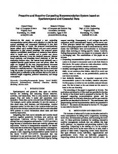
As noticed in the surveys of Davenport and Beck [9] and Herroleen and Leus [11] on scheduling with uncertainty, introducing flexibility in the solutions computed off-line allows to increase the robustness of the system. Hence, we consider that a solution to the problem is not a particular schedule but a set of schedules characterized by a structure defined by a partial order of jobs and a type of schedules. The schedule type can be semi-active, active or non-delay, see for example [5]. For a semi-active schedule, a job cannot be shifted to start earlier without changing the job sequence or violating the feasibility (here precedence constraints and release dates). An active schedule is a schedule where no job can be shifted to start earlier without increasing the completion time of another job or violating the feasibility. A schedule is called nondelay if the machine does not stand idle at any time when there is a job available at this time. Observe that the set of non-delay schedules is a subset of the set of active schedules which is in turn a subset of the set of semi-active schedules. Consider the four job problem shown in table 1 and the partial order where the only restrictions are that job 1 precedes jobs 3 and 4 and job 2 precedes 4. We obtain two non-delay schedules S1 and S2 , three active schedules S1 , S2 and S3 and five semi-active schedules S1 , . . . , S5 , see figure 1. The corresponding objective function values are also given in the same figure. It is clear that proposing several good schedules is more interesting than proposing only one. The decision maker can consequently choose the schedule that better respond to his preferences and possibly to non-

A proactive reactive approach in the presence of disturbances Table 1.

5

A numerical example Job j 1 2 3 4

S1

1

2

rj 0 1 0 9

3

pj 3 3 2 2

1

3

2

2

1

r2 S4

3

11

-

11

-

4 r4

1

11

-

4 r4

S3

2

4

3

2 r2

Figure 1.

1

wj Tj (S1 ) = 0

P

wj Tj (S2 ) = 0

P

wj Tj (S3 ) = 1

P

wj Tj (S4 ) = 4

P

wj Tj (S5 ) = 5

13 4

r4

P

-

r4 S5

wj 1 1 1 1

4 r4

S2

dj 6 8 9 12

3

-

13

Represented non-delay, active and semi-active schedules.

modeled constraints. It is even more interesting if some proposed schedules have common characteristics allowing to switch from a schedule to another easily. In this case, the decision maker can postpone the choice of the schedule to be executed. It is only on-line that he makes this decision taking into account up-to-date information regarding the state of the system. The structure defined by the couple (partial order of jobs, type of schedules) allows to represent several schedules having common precedence constraints between jobs. In order to switch from a schedule to another, or from a subset of schedules to another subset, one or several edges in the disjunctive graph representing the partial order should be oriented without creating cycles in the obtained graph. Furthermore, a partial order is a natural structure used in iterative methods. In such approaches, one or several arcs are added in each step. The use of transitive graphs allows to guarantee the feasibility of the obtained schedule.

6

2.2

Definition of the quality of a solution

The example discussed in subsection 2.1 shows that the quality a priori of a partial order depends on the type of schedules considered. Indeed, for semi-active schedules, there are less restrictions and this allows to obtain five represented schedules instead of two and three for, respectively, non-delay and active schedules. The number of represented schedules can measure the flexibility in job sequencing of a solution. Thus, considering semi-active schedules allows to improve the flexibility of a solution according to the proposed measure. However, the performance of the represented schedules is worse than when considering active or non-delay schedules (see the performance of schedules S4 and S5 ). In our first implementation, we consider that the schedules are restricted to be semi-active. According to this choice, we define in the following the different quality measures of a solution.

2.2.1 sures.

A. Performance of a solution and the associated mea-

A.1. Definition of the performance. Let S be a solution to the problem. It is a partial order that represents a set of semi-active schedules oS . To each schedule oS ∈ S is associated a vector Γ(oS ) = (Γ1 (oS ), Γ2 (oS )), where Γ1 (oS ) is the makespan of oS and Γ2 (oS ) its total weighted tardiness. Hence, a solution S is represented by the set of vectors Γ(oS ). Figure 2 represents the vectors Γ(oS ) in the (Cmax , T¯w ) space.

Figure 2.

The representation of a solution S in (Cmax , T¯w ) space.

The performance of solution S is closely related to the objective function values of all represented schedules oS . Since the number of these schedules can be rather big, it is natural to consider only their most important representatives. We suggest to use only the best and the worst


7

case performances to evaluate the performance of a flexible schedule. The best case performance provides a lower bound of the performance when following the partial order. Whereas, the worst case performance gives a guarantee about how poorly the schedules may perform when following the partial order. They can be obtained by solving corresponding minimization and maximization problems. Hence, we have to determine the coordinates of points A, B, C and D shown in figure 2. The rectangle formed by these points represents the range of the objective function values of all the schedules following the considered solution. We denote by goal point, the point in (Cmax , T¯w ) space whose co∗ ordinates are respectively the best makespan Cmax and the best total ∗ weighted tardiness T¯w of the problem (without the additional precedence constraints brought by the considered partial order), see figure 2. A solution S is all the more efficient that the distance between the goal point to each point A, B, C and D is small. Hence, a performance measure of a solution S can be defined as a linear combination DS of the distances between the goal point and the four points A, B, C and D (see figure 2). These points are determined by computing the best and worst makespan, denoted by BCmax and W Cmax , and best and worst total weighted tardiness, denoted by B T¯w and W T¯w . We have DS = αDS1 + (1 − α)DS2 , where α ∈ [0, 1] and DS1 = β

∗ ∗ BCmax − Cmax W Cmax − Cmax + (1 − β) , β ∈ [0, 1], ∗ ∗ Cmax Cmax

B T¯w − T¯w∗ W T¯w − T¯w∗ + (1 − γ) , γ ∈ [0, 1]. T¯w∗ + 1 T¯w∗ + 1 The lower is DS , the higher the performance of solution S is. DS2 = γ

A.2. Computation of the performance. The objective functions considered are the total weighted tardiness T¯w∗ and the makespan Cmax . It is proved that the problem of minimizing the makespan with respect to precedence constraints, denoted by 1|prec, rj |Cmax , can be solved in O(n2 ) times [13]. The problem P of minimizing the total weighted tardiness, denoted by 1|prec, rj | wj Tj is NP-hard in the strong sense, see for example [14]. Consequently, for this latter problem we implemented a genetic algorithm based heuristic and made comparison with known dynamic dispatching rules like ATC, X-RM and KZRM [17]. The results showed that genetic algorithm we implemented is efficient but is time consuming for a large number of jobs, see [3]. In order to compute the worst makespan and the worst total weighted tardiness which can be reached when considering a partial order S, we

8 introduced in [2] new optimization problems. These are maximization problems denoted by 1(sa)|prec, rj |(F → max), where F is the objective function to be maximized and notation sa means that semi-active schedules are considered. We proved that the problem 1(sa)|prec, rj |(Cmax → P max), can be solved in O(n2 ) times and the problem 1(sa)|prec, rj |( wj Tj → max), is NP-hard in the strong sense [2]. We developed several heuristics based on genetic algorithms and dispatching rules. We obtained the same conclusions as for minimization problems, see [3]. As a result, for a given solution (a set of schedules w.r.t. a partial order), we use polynomial time algorithms to compute the exact minimal and maximal makespan and approximate algorithms based on dispatching rules for estimated minimal and maximal total weighted tardiness.

2.2.2 B. Definition of the flexibility of a solution and the associated measures. One of the main characteristics of a solution to the problem is its flexibility. According to the example presented in the previous subsection, a solution is all the more flexible that the number of represented schedules is great. Indeed, when we have many schedules, it would be possible to dispose on-line, every time a decision has to be taken, of more than one alternative. This could allow to hedge against some perturbations such that raw material availability. This flexibility, called flexibility in job sequencing, can be measured by the number of different schedules feasible with respect to the partial order. However, the problem of calculating this number is #P -complete [7]. Thus, we propose another measure F lexseq equal to the number of non-oriented edges in the transitive graph representing the partial order. If this number is great, then the associated solution is flexible. In our proactive algorithm, we use a transformation of this number into a qualitative scale on several flexibility levels. Each level is defined by an interval [nbArcsM in, nbArcsM ax] giving the minimal and maximal number of arcs that the solution contains. Furthermore, another type of flexibility can be provided according to the time window in which the jobs are executed. This flexibility is called flexibility in time. A measure of this flexibility F lextime can be given by the ratio between the time window in which the jobs can be executed and the total processing time of the jobs: W Cmax − P F lextime = P where W Cmax is the worst makespan of the considered solution and P is the total processing time of all the jobs.


2.3

9

A genetic algorithm to achieve scheduling flexibility

In this section, we present a genetic algorithm used to build-up offline the set of Pareto solutions conciliating good shop performances and flexibility presence. These solutions are determined by an exploration of the whole solution space. In practice, this exploration may be limited to a sub-space of solutions satisfying possible preferences of the decision maker. These preferences are accounted of thanks to an interactive support decision tool which is not presented in this paper. In the following, we present the general scheme of the genetic algorithm we implemented. Then, we describe the selection and reproduction strategies, the encoding used to represent a solution to the problem (partial order) and the genetic operators, crossover and mutation, that generate new solutions.

2.3.1 A. General scheme of the genetic algorithm. The aim of this algorithm is to generate for a given problem a set of solutions, which yield a good compromise between flexibility and performance. According to the previous section, a solution S is all the more good that the distance Ds (S) is minimal, the flexibility in job sequencing f lexseq (S) is maximal, the flexibility in time f lextime (S) is maximal. The principle of the algorithm is to work on different populations of solutions that belong to a same level of flexibility in job sequencing. Recall that a level of flexibility is defined by an interval [nbArcsM in, nbArcsM ax] giving the minimal and maximal number of arcs that a solution can contain. The objective is to find, in the space of solutions that belong to the same level of the flexibility in job sequencing, the solutions realizing a good compromise between the performance (measured by Ds ) and the flexibility in time (measured by F lextime ). We use a linear combination of these two criteria to compute the fitness of a chromosome representing a solution S. F itness(S) = θDs (S) − (1 − θ)F lextime (S), where θ ∈ [0, 1]. For a fixed parameter θ, the algorithm works as described in figure 3. In this algorithm, we use the following notations : nbGen is the number of generations ; Pi is the population of individuals in iteration i = 1, . . . , nbGen; nbLevels is the number of levels of flexibility in job sequencing ;

10 EliteLl ,θ , is the elite population obtained at the end of the algorithm for a fixed value θ ∈ [0, 1] and for the level of flexibility in job sequencing Ll , l = 1, . . . , nbLevels.

For l = 1 to nbLevels do Generate a population of solutions P0 belonging to a level of flexibility in job sequencing Ll ; Evaluate the chromosomes in P0 and initialize EliteLl ,θ ; For i = 0 to nbGen do Select Npop couples of chromosomes for reproduction; Cross the selected couples of chromosomes; Evaluate the generated children and update EliteLl ,θ ; Mutate with a small probability πmut the generated children; Evaluate the mutated children and update EliteLl ,θ ; Select Npop chromosomes from Pi and the generated children; EndFor EndFor

Figure 3.

The genetic algorithm for a fixed value of θ

In order to find the Pareto optimal solution set of this multi-criteria problem, we vary the value of θ between 0 and 1 and apply the previous algorithm for each value of θ.

2.3.2 B. Selection and reproduction strategy. In each iteration of the genetic algorithm, we use two selection procedures. The first selects Npop couples of chromosomes for reproduction. The second selection procedure selects, among the generated children and the old population, Npop chromosomes that will survive and form the new population Our implementation uses the roulette selection by rank for the two previous procedures. Denote by NpopIn the number of chromosomes of the initial population from which the procedure selects NpopOut chromosomes for reproduction or survival. The best chromosome is affected a new fitness equal to NpopIn , the second best chromosome a fitness equal to NpopIn − 1 and the last one a fitness equal to 1. The chromosomes are selected with a chance proportional to their rank. The roulette selection works as described in figure 4. 2.3.3 C. Encoding. In order to encode a given solution S (partial order), we use a ternary precedence constraint oriented matrix A, which represents the set of


11

Sort the initial population of NpopIn chromosomes in the non decreasing order of their fitness; set f0 = 0; For i = 1 to NpopIn do 2(N −i) set fi = fi−1 + NpopInpopIn ; (NpopIn +1) EndFor For i = 1 to NpopOut do Choose randomly a real π ∈ [0, 1[; Select the chromosome i∗ such that fi∗ −1 ≤ π < fi∗ ; EndFor

Figure 4.

The roulette selection by rank

precedence constraints contained in the transitive graph representing the partial order. This matrix A = (aij )1≤i,j≤n is defined as follows:   1 aij = −1   0

if job i precedes job j, if job j precedes job i, if i = j or i and j are permutable.

This matrix is transitive and anti-symmetric. Only n(n − 1)/2 elements are kept inside the computer memory, but the complete matrix is used here for clarity sake. It is a direct encoding because there is a one-to-one correspondence between the ternary matrix space and the solution space [10, 18].

Example 1. Consider a five job problem. A solution to this problem is given by the partial order represented in figure 5. In this solution, the only restrictions are that job 2 precedes jobs 3,4 and 5; and job 4 precedes job 3. This solution represents 15 schedules. It is encoded by the ternary matrix given in figure 5.

Figure 5.

A solution and the corresponding encoding

12 2.3.4 D. Modified MT3 crossover. In order to generate two children from two mates, we use an adaptation of the crossover MT3 proposed by Djerid and Portmann [10], which was used for job shop scheduling problem. Consider two mates (Mate 1 and Mate2) represented respectively by matrix A1 and matrix A2 . The algorithm corresponding to the crossover that generates the first child, represented by matrix F , works as described in figure 6. 1

2

Step 1.

Compute F = A +A ;//integer division: the value is truncated 2 to 0 when obtaining 12 or − 12 Update nbArcs(F );

Step 2.

Make a decision on the value of one fij to ensure, if possible, that the child will be different from both mates ; Update nbArcs(F );

Step 3.

While nbArcs(F ) < nbArcs(A1 ) do Select randomly mate 1 with probability π or mate 2 with probability 1 − π; Select randomly two jobs i and j such that fij = 0 and aij 6= 0;//A is the matrix of the selected mate set fij = aij ; set fji = −fij ; Compute the transitive closure of F and update nbArcs(F ); EndWhile

Step 4.

if nbArcs(F ) ≤ nbArcsM ax then F is kept ; else F is discarded ;

Figure 6.

The modified MT3 crossover

Step 1 allows to keep the common precedence constraints in the two parents. In step 3, we add 1 and −1 (precedence constraints) in the matrix of the child according to the parents until reaching nbArcs(A1 ) (or nbArcs(A2 )). The probability π, which we choose equal to 0.6 in the implementation of the algorithm, allows that child 1 (resp. child 2) resembles more to mate 1 (resp. mate 2). In figure 7, we present an example that illustrates the proposed crossover.

Remarks. The crossover presented below guarantees an interesting property that is: if i precedes j in both mate 1 and mate 2, then i precedes j


Figure 7.

13

MT3 crossover - example

in the generated offspring. It allows to keep the important properties of a good solution. Furthermore, it guarantees that imperative precedence constraints, if they exist, are usually respected. If the obtained offspring F is such that nbArcs(F ) > nbArcsM ax, then we can withdraw the obtained solution and reiterate or try to eliminate some arcs in order to obtain nbArcs(F ) almost equal to nbArcsM ax. Unlike the crossover proposed by Djerid and Portmann [10], the presented crossover stops adding 1 and −1 when the number of arcs in the generated offspring reaches the number of arcs of the corresponding mate. Besides, step 2 is used to ensure that the generated child is different from his parents. This step is motivated by the chosen scheme of the genetic algorithm: Davis reproduction.

14 2.3.5 E. MUT3 Mutation. The mutation operator is used to guarantee the diversity of the population of chromosomes. The mutation we propose consists in changing the order of at least two jobs. It is described in figure 8, where A is the matrix of the considered mate. Step 1.

Initialize F = F0 ; /* F0 is the matrix representing the imposed precedence constraints */

Step 2.

Select randomly two jobs i and j such that aij 6= 0; set fij = −aij ; set fji = −fij ; While nbArc(F ) < nbArc(A) Select randomly two jobs i and j such that fij = 0 and aij 6= 0; set fij = aij ; set fji = −fij ; Compute the transitive closure of F ; EndWhile

Step 3.

if nbArcs(F ) ≤ nbArcsM ax then F is kept ; else F is discarded ;

Figure 8.

3.

The mutation MUT3

The reactive algorithm

The reactive algorithm has three important roles. The first is to make the remaining scheduling decisions on-line w.r.t the precedence constraints imposed by the chosen partial order. The second role is to react when a perturbation occurs. The third role is to detect when the solution in use is infeasible with respect to the decision maker objectives. A reactive algorithm is efficient if it allows 1 to offer if possible, every time a decision has to be made, more than one alternative with respect to the partial order and consequently be able to absorb possible late arrival of raw material, 2 to exploit the flexibility in time when a machine breaks down, and 3 to obtain good performance for the realized schedule. Clearly, it is impossible to satisfy these objectives simultaneously.

15


We designed different procedures to achieve an acceptable compromise between the aforementioned objectives. In the remainder of the paper, the following notations are used. For a set of jobs X, X + is the subset of available jobs. A job is available if all its predecessors (w.r.t. the partial order) are scheduled and if it satisfies the restrictions on the constructed schedules (semi-active, active or non-delay schedules). P RIOR1 (i, t) and P RIOR2 (i, t) are two functions that give the priority of a job i at time t. The general scheme of the reactive algorithms we propose is given in figure 9. At a given time t, the algorithms schedule the job i∗ that maximizes P RIOR1 (i, t) among the available jobs i, i.e., i ∈ X + . When two or more jobs are in competition, the job that maximizes P RIOR2 (i, t) is selected. Set X = N and t = 0; While X 6= φ do Determine X + ; Determine the set Y1 = {i ∈ X + , P RIOR1 (i, t) maxj∈X + {P RIOR1 (j, t)}}; Select a job i∗ ∈ Y1 such that P RIOR2 (i∗ , t) maxj∈Y1 {P RIOR2 (j, t)}}; Set X = X\{i∗ }; Set t = max{t, ri∗ } + pi∗ ; endWhile

Figure 9.

= =

The general scheme of the proposed algorithms

Clearly, the algorithms depend on the priority functions P RIOR1 (i, t) and P RIOR2 (i, t). They also depend on the definition of the job availability. Indeed, even though the partial order was computed off-line while considering that the represented schedules are semi-active, we may decide on-line to construct active or non-delay schedules for a performance improving purpose. When a disruption occurs, an analysis module is used. In the case of a breakdown, this module uses some results developed in [1] to compute an upper bound of the increase on the worst total weighted tardiness and to possibly propose one or several decisions to minimize it. The increase on the worst makespan can be computed with a polynomial time algorithm [2]. We consider now the second type of disruptions : late

16 job arrival. Suppose that, at time t, the algorithm chooses to schedule a disrupted job j such that rjm > t, where rjm is the new release date of the job. If there exists an available non-disrupted job i, it can be scheduled without any increase on the worst case objective function’s values. If such a job does not exist, then this perturbation can be considered as a breakdown and an upper bound of the increase on the worst total weighted tardiness can be computed. When the loss of performance is too important, we can either restrain the partial order in order to have an acceptable increase or recalculate a new solution (partial order) for the remaining non scheduled jobs.

4.

Computational results

We conducted several experiments to evaluate the proactive algorithm and the use of the proposed approach both in deterministic and stochastic shop conditions. The first type of experiments concerns the proactive algorithm and its ability to construct solutions providing a good tradeoff between the measures of flexibility and performance. The experiments proved that the genetic algorithm allows to provide an acceptable trade-off between flexibility and performance when the dispersion of job arrival is not very high. Otherwise, the job permutation is penalizing [1]. In the second type of experiments, we tested the application of the approach in deterministic shop conditions. We proved that the best two algorithms in deterministic shop conditions are P erf N D and F lex1 N D. P erf N D constructs non-delay (ND) schedules using ATC heuristic as the first priority function (P RIOR1 (i, t)) and the non-decreasing order of release dates as the second priority function (P RIOR2 (i, t)). F lex1 N D tries to maximize the use of the flexibility in job sequencing contained in the considered solution by maximizing the number of possible choices in the following step. The second priority rule is ATC [1]. In this paper, only experiments in stochastic shop conditions case are detailed.

4.1

Experimentations in stochastic shop conditions

In order to evaluate the proposed proactive reactive approach, we compare it to a predictive reactive approach. In this predictive reactive approach, a predictive schedule is computed using KZRM heuristic without taking into account the presence of future disruptions. This schedule is then proposed to the shop for execution. When a disruption occurs, a reactive algorithm, based on ATC heuristic, is used to compute a new schedule with respect to the current state of the system.


17

Theoretically, we can expect that the predictive reactive approach outperforms our proactive reactive approach. Indeed, we use a simple reactive algorithm which allows only small modifications on the partial order characterizing the retained solution. Besides, it was proved that ATC heuristic constructs good schedules compared to optimal schedules [12]. However, as it is shown in the following subsections, our proactive reactive approach has a better behavior when disruptions have low or medium amplitude.

4.1.1 Description. The context of our experimentations is the following. We consider that, in order to produce a final product, two components are needed: a principal component and a secondary component. The principal components are delivered by an upstream shop. The release dates rj of the jobs, used by the proactive and predictive algorithms, are equal to the arrival dates of the corresponding components. The secondary components are bought and used for the transformation of the principal components. We suppose that two different principal components do not need the same secondary components. After acquisition, the secondary components are stored in the shop until their use. We associate to each secondary component a storage cost proportional to its storage duration. The obtained products are then delivered to a downstream shop. A penalty is associated to each job if it is tardy with respect to the due dates dj given by the downstream shop. Two solutions S pro and S pred are computed off-line using, respectively, the proactive algorithm and the predictive algorithm. The computation of these solutions takes into account the delivery time of principal components rj and the due dates dj . In order to minimize the cost of secondary component storage, the purchase date of these components is a function of the starting time of the corresponding principal products in S pro or S pred . The finishing time of the principal component can determine their new delivery dates that can be communicated to the downstream shop. A penalty is also associated to each job if it is tardy with respect to the new delivery dates. The following notations are used (see figure 10). For each job j, we denote by: pj its processing time;

18 tjpred its starting time in S pred ; t1jpro its earliest starting time with respect to the partial order defining S pro ; t2jpro its latest starting time with respect to the partial order defining S pro (j is placed just before its successors [2]); tjef f its effective starting time in the realized schedule Sr ; sj the acquisition date of the secondary component used to produce j. It is given by the following: ( ti − θ1 for the predictive reactive approach si = 1pred (1) tipro for the proactive reactive approach where θ1 is a constant (see figure 10). dj its due date asked by the downstream shop; δi its new delivery date given by the following: ( ti + pi + θ2 = δipred for the predictive reactive approach δi = 2pred tipro + pi = δipro for the proactive reactive approach (2) where θ2 is a constant (see figure 10). Tj (resp. Tjδ ) is the tardiness of j with respect to dj (resp. δj ). The performance of the realized schedule Sr is function of three measures: the storage cost storageCost(Sr ) and the tardiness W T (Sr ) with respect to the due dates dj and the tardiness W T δ (Sr ) with respect to the delivery dates δj . These measures are given by the following equations : X storageCost(Sr ) = c(tief f − si ), (3) i∈N

where c is the unitary storage cost. X X W T (Sr ) = wi Ti = wi max(0, tief f + pi − di ). i∈N

W T δ (Sr ) =

X i∈N

(4)

i∈N

wi Tiδ =

X i∈N

wi max(0, tief f + pi − δi ),

(5)


19

Figure 10. The different parameters for a job i in the proactive solution, the predictive schedule and the realized schedule

To be fair to the predictive approach, constants θ1 and θ2 are chosen in such a way that the predictive schedule S pred is given a flexibility equivalent to the flexibility contained in the proactive solution S pro . Constant θ1 is such that the obtained storage costs are equivalent when considering S pro or S pred . The value of θ2 is such that X i∈N

(δipro − di ) ≈

X

(δipred − di )

(6)

i∈N

4.1.2 Problem’s generation scheme. The generation scheme is the one used by Mehta and Uzsoy [16]. The job’s number is equal to 40. The processing times pj are generated from a discrete uniform distribution U nif orm(pmin , pmax ). The job release times rj are generated by a discrete uniform distribution between 0 and ρnpav , where pav is the expected processing time. The parameter ρ controls the rate of job arrivals. The job due dates dj are generated as dj = rj + γpav , γ is generated from a continuous distribution U nif orm[a, b]. The job weights wj are either all equal to 1 or generated by a discrete uniform distribution between 1 and 10. 4.1.3 Disruption’s generation scheme. Two types of disruptions are considered: machine breakdowns and late arrival of principal components (increase of some rj ). The breakdowns are characterized by their occurrence time and their duration. The number of breakdowns is denoted by nbBreak. The scheduling horizon is divided into

20 equal nbBreak intervals such that in each interval a breakdown occurs. The breakdown durations are generated from a uniform distribution U nif orm(durM in, durM ax). The disruptions related to late arrival of the principal components are generated according to the considered predictive schedule or proactive solution. When using a predictive schedule S pred , a perturbation is generated by associating a new earliest starting time rjm = tjpred + aug, where tjpred is the starting time of job j in S pred and aug is generated from a uniform distribution U nif orm(augM in, augM ax). When considering a proactive solution S pro , rjm = t1jpro + aug, where t1jpro is the earliest starting time of job j with respect to the partial order defining S pro . For each problem, we consider a proactive solution and a predictive schedule to be compared. About 50% of disruptions related to late raw material arrival are generated according to the predictive schedule and 50% according to the proactive solution. The number of delayed jobs is denoted nbDelay.

4.2

Analysis of the obtained results

We implement two heuristics of the reactive algorithm in the predictive reactive approach : AT C di and AT C δi . These are ATC based heuristics that construct non-delay schedules. The first takes into account the due dates di and the second the delivery dates δi . For the proactive reactive approach, we use heuristics P erf N D and F lex1 N D presented in section 3. The comparison is based on the criteria W T and W T δ given respectively by equations (4) and (5). The performance is measured by evaluating W T + W T δ . We consider the following parameters to generate problems and disruptions. (pmin , pmax ) = (1, 11), ρ = 0.5, 1 : grouped or dispersed job arrivals, (a, b) = (1, 3) or (2, 5) to generate the due dates. For the four parameter combinations, we generate five problems. For each problem, we use KZRM heuristic to generate a predictive schedule and the proactive algorithm to compute a flexible solution belonging to the flexibility level characterized by nbArcs ∈ [620, 700]. Then, these solutions are executed subject to disruptions characterized by the following parameters. The number of breakdowns nbBreak ∈ {0, 1, 2, 3};


21

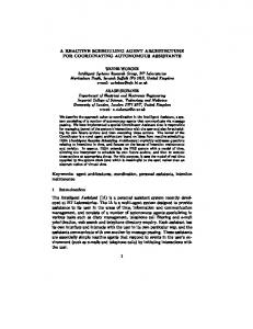
[durM in, durM ax] = [3, 6] for breakdown durations; [augM in, augM ax] ∈ {[1, 6], [6, 12], [12, 24], [24, 36], [36, 48], [60, 90]}; nbDelay ∈ {4, 6, 8} For each combination of these parameters, a couple (predictive schedule, proactive solution) is experimented in 1000 different scenarii. The performance of each reactive algorithm F lex1 N D, P erf N D, AT C di and AT C δi in terms of total weighted tardiness is evaluated for each scenarii. The average value is then computed and associated to each algorithm. The reactive algorithm with best performance is assigned a performance equal to 100%. Any of the three remaining algorithms is assigned the ratio between the best performance and its performance. Figures 11, 12, 13 et 14 sum up the obtained results for the family of problems corresponding to ρ = 0.50, (a, b) = (1, 3), nbDelay = 8 and nbBreak = 0, 1, 2, 3 and the proactive solution is characterized nbArcs = 680. We can notice that algorithms AT C di and AT C δi are dominated by algorithms F lex1 N D and P erf N D for late arrival disruptions characterized by [augM in, augM ax] ∈ {[1, 6], [6, 12], [12, 24], [24, 36]}. The superiority of F lex1 N D and P erf N D is very clear when nbBreak = 2. For important late arrival disruptions, notably when [augM in, augM ax] = [60, 90], the performance of F lex1 N D and P erf N D become less than 86%. Besides, in all cases P erf N D outperforms F lex1 N D. This is also the case for AT C δi when compared to AT C di . We obtain the same conclusions when (a, b) = (2, 5) . We applied the same experimentations for more flexible solutions characterized by nbArcs ≈ 540. We remarked that algorithms F lex1 N D and P erf N D becomes rapidly dominated by algorithms AT C δi and AT C di . When the dispersion of job arrival is high (ρ = 1.00), our algorithms F lex1 N D and P erf N D outperform the other algorithms when the level of disruptions on job arrival is low ([augM in, augM ax] ≤ [12, 24]) and nbBreak = 0 or 1. When the number of breakdowns is greater, notably for nbBreak = 2, the performance of AT C δi and AT C di are less than 50%. Besides, in all cases P erf N D outperforms F lex1 N D. This is also the case for AT C δi when compared to AT C di . To summarize, when the job arrivals are grouped (ρ = 0.50), our approach is usually superior to the predictive reactive approach when the amplitudes of disruptions on job arrival are such that [augM in, augM ax] ≤ [36, 48] and nbBreak = 0, 1, 2, 3. For dispersed job arrivals (ρ = 1.00), our approach is very superior when nbBreak ≥ 2.

22

Figure 11. Results for (pmin , pmax ) = (1, 11), ρ = 0.50, (a, b) = (1, 3), nbArcs = 680, nbDelay = 8 et nbBreak = 0.



23



24 When nbBreak < 2, it also outperforms the other approach for disruptions on job arrival with low amplitude. In conclusion, according to the experiments presented in this paper, our proactive reactive approach outperforms a predictive reactive approach for low and medium disruption amplitude.

5.

Conclusion

We considered in this paper the single machine scheduling problem with dynamic job arrival and total weighted tardiness and makespan as objective functions. The shop environment is subject to perturbations related to late raw material arrival and to machine breakdowns. We proposed a proactive reactive approach to solve the problem. The proactive algorithm is a genetic algorithm which computes partial orders providing a good trade-off between flexibility and performance. These solutions are built up while taking into account the shop constraints, the decision maker preferences and some knowledge about possible future perturbations. The reactive algorithm is used to guide on-line the execution of the jobs. In the presence of disruptions, the reactive algorithm is used to absorb their effects by exploiting the flexibility introduced in the proactive algorithm. We made several experimentations to compare our approach to a predictive reactive approach in stochastic shop conditions. The results showed that our approach outperform the predictive reactive approach for low and medium disruption amplitude. This confirms that anticipating the presence of disruptions proactively allows to obtain good realized schedules and to plan other shop activities. The results obtained for single machine scheduling problems gave us some insight to extend our approach to more complex scheduling problems. Currently, we are adapting the proposed proactive algorithm for flow shop scheduling problem with maximum cost functions. A solution to this problem is characterized by a partial order on each machine. This extension is motivated by a polynomial time algorithm developed in [1] to compute the worst case performance for the flow shop case.

References [1] M.A. Aloulou. Structure flexible d’ordonnancements ` a performances contrˆ olées pour le pilotage d’atelier en présence de perturbations. PhD thesis, Institut National Polytechnique de Lorraine, December 2002. [2] M.A. Aloulou, M.Y. Kovalyov, and M.C. Portmann. Maximization in single machine scheduling. Annals of Operations Research, accepted for publication by the guest editors, 2003. [3] M.A. Aloulou and M.C. Portmann. Incorporating flexibility in job sequencing for the single machine total weighted tardiness problem with release dates. In


25

10th Annual Industrial Engineering Research Conference, pages in CD–ROM. IIE, May 2001. [4] C. Artigues, F. Roubellat, and J.-C. Billaut. Characterization of a set of schedules in a resource constrained multi-project scheduling problem with multiple modes. International Journal of Industrial Engineering, Applications and Practice, 6:112–122, 1999. [5] K.R. Baker. Introduction to Sequencing and Scheduling. John Wiley and Sons, 1974. [6] J.C. Billaut and F. Roubellat. A new method for workshop real time scheduling. International Journal of Production Research, 34(6):1555–1579, june 1996. [7] G. Brightwell and P. Winkler. Counting linear extensions. Order, 8:225–242, 1991. [8] L.K. Church and R. Uzsoy. Analysis of periodic and event-drive rescheduling policies in dynamic shops. International Journal of Computer Integrated Manufacturing, 5:153–163, 1992. [9] A.J. Davenport and J.C. Beck. A survey of techniques for scheduling with uncertainty. http://www.eil.utoronto.ca/profiles/chris/chris.papers.html, 2000. [10] L. Djerid and M.C. Portmann. Genetic algorithm operators restricted to precedent constraint sets : genetic algorithm designs with or without branch and bound approach for solving scheduling problems with disjunctive constraints. In Proceedings of IEEE International Conference on Systems, Man and Cybernetics, volume 4, pages 2922–2927, October 14-17 1996. [11] W. Herroelen and R. Leus. Project scheduling under uncertainty survey and research potentials. Invited paper in a special issue of the European Journal of Operational Research, 2003. to appear. [12] A. Jouglet. Ordonnancer sur une machine pour minimiser la somme des coˆ ut. PhD thesis, Université de Technologie de Compiègne, November 2002. [13] E.L. Lawler. Optimal sequencing of a single machine subject to precedence constraints. Management Science, 1973. [14] E.L. Lawler, J.K. Lenstra, A.H.G. Rinnooy Kan, and D.B. Shmoys. Logistics of Production and Inventory, Handbook in Operations Research and Management Science 4, chapter Sequencing and scheduling: algorithms and complexity, pages 445–452. 1993. [15] V.J. Leon, S.D. Wu, and R.H. Storer. Robustness measures and robust scheduling for job shops. IIE Transactions, 26(5):32–43, 1994. [16] S.V. Mehta and R. Uzsoy. Predictable scheduling of a single machine subject to breakdowns. International Journal of Computer Integrated Manufacturing, 12:15–38, 1999. [17] T.E. Morton and D.W. Pentico. Heuristic Scheduling with Apllications to Production Systems and Project Management. Wiley, New York, 1993. [18] M.C. Portmann, A. Vignier, C.D. Dardilhac, and D. Dezalay. Branch and bound crossed with ga to solve hybrid flowshops. European Journal of Operational Research, 107:389–400, 1998. [19] G.E. Vieira, J.W. Herrmann, and E. Lin. Rescheduling manufacturing systems: a framework of strategies, policies, and methods. Journal of Scheduling, 6(1):35– 58, 2003.

26 [20] S.D. Wu, E.S. Byeon, and R.H. Storer. A graph-theoretic decomposition of the job shop scheduling problem to achieve scheduling robustness. Operations Research, 47(1):113–124, 1999.