An Efficient Scheduling Mechanism for IEEE 802.11E MAC Enhancements Shou-Chih Lo
Wen-Tsuen Chen
Dept. of Computer Science National Tsing Hua University HsinChu, Taiwan, R.O.C.
[email protected]
Dept. of Computer Science National Tsing Hua University HsinChu, Taiwan, R.O.C.
[email protected]
Abstract—To guarantee the delay and jitter bounds for real-time traffic, the polling scheme is commonly used in the IEEE 802.11 medium access control (MAC) protocol. However, the polling overhead becomes significant when continuous and periodic realtime traffic is served. We propose a scheduling mechanism by which wireless stations can issue their frame transmissions automatically without too much indication from the system. The system can initiate a scheduling access phase (SAP) on the channel at anytime during which the scheduled stations can do data transmissions. We specify the transmissions of wireless stations being scheduled in a way of ordered contentions within the SAP. The contending feature can bring the advantages of easy implementation and high channel utilization. Keywords-Wireless LAN; MAC; QoS; Polling; Scheduling
I.
INTRODUCTION
IEEE 802.11 [10] is an international Wireless Local Area Network (WLAN) standard. The 802.11 WLAN consists of Basic Service Sets (BSS), each of which is composed of wireless stations (STA). The WLAN can be configured as an ad hoc network (an independent BSS) or an infrastructure network (composed of an access point and the associated STAs). The channel access for the STAs in a BSS is under the control of a coordination function. The 802.11 WLAN provides two coordination functions: Distributed Coordination Function (DCF) and Point Coordination Function (PCF). The DCF is a contention-based access scheme using Carrier Sense Multiple Access with Collision Avoidance (CSMA/CA). Priority levels for access to the channel are provided through the use of Interframe Spaces such as SIFS, PIFS and DIFS. The backoff procedure is used for collision avoidance, where each STA waits for a backoff time (a random time interval in units of a slot time) before each frame transmission. The performance analysis of the DCF was studied in [1][2][3][5]. The PCF provides contention-free transmission in an infrastructure network by using the Point Coordinator (PC) to poll each STA in turn. The DCF and the PCF can coexist by alternating the Contention Period (CP), during which the DCF is performed, and the Contention-Free Period (CFP), during which the PCF is performed. A CFP and a CP are together referred to as a CFP Repetition Interval or a Superframe.
This research was partially supported by the Educational Ministry of the Republic of China under Contract No. 89-E-FA04-1-4.
To expand support for applications with quality-of-service (QoS) requirements, the IEEE 802.11E task group is proceeding to build the QoS enhancements of the 802.11 Medium Access Control (MAC) protocol. In the 802.11E draft [11], the Hybrid Coordination Function (HCF) was proposed. The HCF uses a contention-based channel access method (called enhanced DCF, EDCF) to provide the prioritized data delivery, and uses a controlled channel access method to provide the parameterized data delivery. In the EDCF, each traffic flow will be assigned with a different backoff time whose value decreases with increasing traffic priority. In the HCF controlled channel access, an STA can be guaranteed to issue the frame transmission even during the CP by using the Controlled Access Phase (CAP). The CAP can be viewed as a temporary CFP, during which the transmissions of STAs are coordinated by the poll-based scheme as in the PCF. The benefit and the performance of the IEEE 802.11E MAC were studied in [8][14]. II.
MOTIVATION
Real-time traffic is usually associated with QoS requirements like delay and jitter bounds. Using a centralized coordinator to schedule the transmissions of real-time flows can properly meet their requirements. The polling scheme is a common technique to coordinate the transmissions of real-time flows in the IEEE 802.11 WLAN. In the PCF, the PC maintains a polling list and polls each STA by sending a polling frame (CF-Poll frame) according to the polling list during the CFP. Different polling schedules were studied in [4][5][6][9][15]. However, the polling scheme has the drawback of low channel throughput due to the overhead of polling frames. In [13], we propose a multipolling mechanism to reduce the overhead of polling frames by polling several STAs at a time. However, the proposed scheme is suitable for aperiodic real-time traffic. For continuous and periodic traffic like video transmissions, a constant polling on this kind of traffic in the sequential superframes is performed if the PCF or the HCF is used. As a result, the polling overhead becomes significant for the isochronous traffic. If an STA with isochronous traffic can automatically initiate its frame transmission in the sequential superframes without too much indication from the PC, the control overhead can be reduced. A scheduling mechanism
Superframe CFP
Superframe CP
CFP
SIFS
CP
SIFS
TXOP A
SIFS Slot
TXOP A
TXOP B
A's frames
A's frames
B's frames
backoff time 0
backoff time 0
CP-Schedule(B)
≈
≈
CP-Schedule(A)
backoff time 1
Figure 1. Example of CP-Schedule.
(called CF-Schedule) [7] has ever been discussed in the IEEE 802.11E task group. In the CF-Schedule, an STA is allocated with a permanent time interval in the some number of sequential superframes to issue its frame transmissions. The time interval is specified by the Transmission Opportunity (TXOP) that is defined by a starting time and a maximum length. The PC can grant permanent TXOPs to several scheduled STAs together using a single CF-Schedule frame. However, the CF-Schedule has the following problems which make this scheme unpractical. Waste of channel space. Once a scheduled STA fails to receive the CF-Schedule frame due to channel errors or a move into one other BSS, the TXOP allocated to this STA becomes wasted. Also, a scheduled STA may not fully utilize the allocated TXOP when there are not enough pending data to be transferred. Rescheduling overhead. The unpredictable traffic from broadcast or multicast at the beginning of a superframe may affect the starting of scheduled TXOPs. To avoid this problem, the PC has to notify the scheduled STAs the precise staring time by sending the CF-Schedule frame again. On the other hand, the lifetime of each scheduled TXOP is different, so the scheduled TXOPs that are still alive may sparsely distribute over the channel space after a certain time period. It becomes an overhead for the PC to rearrange the scheduled TXOPs. III.
CONTENTION-BASED SCHEDULING MECHANISM
Here, we propose an efficient scheduling mechanism with the advantages of easy maintenance and high channel utilization. The proposed mechanism which is called Contention-Period Schedule (CP-Schedule) incorporates the DCF access scheme into the scheduling scheme. A. Basic Idea In the CP-Schedule, we specify the transmissions of scheduled STAs by using ordered contentions instead of precise time intervals. That is, we specify a distinct backoff time to each scheduled STA in the CP-Schedule frame. These scheduled STAs will contend the channel access based on the access rule similar to the DCF after informed with the starting of contention. The scheduled STAs will win the channel contention in the same order as specified in the CP-Schedule frame if the backoff time is assigned incrementally. The backoff procedure performed here is a little bit different from the one performed in the DCF. The scheduled
STA initiates the decrement of backoff time after a SIFS period rather than a DIFS period when the channel is detected idle. We call it the restricted backoff procedure. Since SIFS < DIFS, this can increase the chance for a scheduled STA to win the channel contention than those STAs from other BSSs in the vicinity of the scheduled STA. A simple example of the CP-Schedule is shown in Fig. 1. STA A with backoff time 0 initiates its activity in the first superframe, while STA B with backoff time 1 initiates its activity in the second superframe. STA A will continue contending the channel access in the second superframe after receiving the CP-Schedule frame. The CP-Schedule has the following advantages. A scheduled STA can hold the channel access flexibly depending on the size of local buffered data, so it becomes easy to deal with the data burst. If a scheduled STA does not fully utilize the allocated TXOP or even makes no response to the CPSchedule, other scheduled STAs will detect the channel idle right away and advance the starting of channel contention. The rescheduling work becomes simple by just changing the backoff time assignment. B. Hidden Terminal Problem Since any two of scheduled STAs in the BSS might not listen to each other when contending the channel access, a collision may occur (known as the hidden terminal problem [5]). Two approaches can be adopted to deal with this problem. One approach is to exploit the capture phenomena [15] in the radio channels, where a transmission with a strong signal can be successfully received even in the present of one other weaker signal. When the PC detects the first data transmission of a scheduled STA, it starts transmitting a jam by a weaker signal till the data frame is completely received. The jamming signal can imply the on-going transmission of one scheduled STA to other scheduled ones. Hence, the other scheduled STAs, whether they are hidden terminals or not, will defer their channel accesses due to the channel busy state. After the jamming, the remaining transmission time of the on-going scheduled STA is protected by the Network Allocation Vector (NAV). The duration time for a frame exchange sequence will be carried in the data and ACK frames. Other contending STAs will wait for the completion of the current frame exchange by updating their NAVs. A scenario example is shown in Fig. 2, where the first scheduled STA is assigned with backoff time 0. When the first scheduled STA is transmitting its first data frame, other scheduled STAs will
detect the channel busy due to the jamming signal or the ongoing data transmission. SIFS
CP-Schedule
SIFS
Jam
SIFS
SIFS
ACK
ACK
PC Data
scheduled and how long these STAs are served. The AID subfield contains an association identifier which identifies an STA in the BSS. The Backoff subfield specifies the backoff time value. The TXOP Limit subfield specifies the maximal duration of a scheduled TXOP. The TXOP Lifetime specifies the maximum number of superframes during which a STA may use its scheduled TXOP.
Data octets: 2
First Scheduled STA Defer(Busy)
NAV(ACK)
Frame Control
2
6
2
Duration BSSID Record /ID Count AID
Other Scheduled STAs
(0-255)
Figure 2.
Jamming approach.
8×RecordCount
4
Schedule Record (8 octets)
FCS
Backoff
TXOP TXOP Limit Lifetime (2 octets) (2 octets) (2 octets) (2 octets)
Figure 4. The frame format of the CP-Schedule frame. SIFS
SIFS
CP-Schedule
SIFS
SIFS
CTS
ACK
PC RTS
Data
First Scheduled STA NAV(RTS) Other Scheduled STAs
NAV(CTS)
Figure 3. RTS/CTS approach.
One variation of the jamming approach is to use the busy tone [16] in multi-channel environments. During the data transmission of one scheduled STA, the PC repeatedly sends a busy tone on the control channel to indicate the busy state of the data channel. Other scheduled STAs will defer their data transmissions on the data channel until the end of the busy tone on the control channel. The other approach is to use the RTS (Request To Send)/CTS (Clear to Send) handshake to deal with the hidden terminal problem. After the scheduled STA wins the channel contention, it should exchange the RTS/CTS frames with the PC. The RTS/CTS frames will carry the duration information. A scenario example is shown in Fig. 3. It is noticed that other scheduled STAs, which are hidden terminals, cannot transmit any frame in the middle of the current transmission of the RTS frame. To guarantee this condition, the gap between backoff time values assigned to two successive scheduled STAs should be large enough to accommodate the time to transmit an RTS frame. By comparison, the jamming approach can avoid the overhead incurred by the RTS/CTS handshake. However, this approach has one restriction that the PC should operate in a non-overlapping channel and a BSS is free from the interference from other wireless networks nearby (e.g. Bluetooth). This environment is available when deploying the IEEE 802.11a WLAN which has several channels available and operates in the 5 GHz frequency band. When this prerequisite is not satisfied, we can return to the approach of using the RTS/CTS handshake. C. Mechanism Design The frame format of the CP-Schedule frame is shown in Fig. 4. The Schedule Record field specifies which STAs are
In the jamming approach, we can assign the backoff time bti to the ith scheduled STA by following the rule: bt1 = 0 and bti = bti-1 + 1 for i ≥ 2. In the RTS/CTS approach, there might have a possible collision between any two scheduled STAs from different BSSs if multiple PCs are operating on the same channel in the overlapping area. To avoid assigning the same backoff time values in the CP-Schedule among neighboring BSSs, two approaches can be used. One is to use the Inter Access Point Protocol (IAPP) discussed in the IEEE 802.11F task group [12] to coordinate the backoff time assignment. The other is to use a distributed algorithm as introduced below. Let h denote the number of PCs operating in the overlapping area. seed is a random number from the interval [0, h-1]. The backoff time assignment follows the rule: bti = seed + h(i−1) for i ≥ 1. If the condition bti − bti-1 ≥ tRTS (the time to transmit an RTS frame) is not satisfied, a simple shift operation on the corresponding backoff time values will be performed. Since the lifetime of each scheduled STA is different, the gap on the backoff time values between two successive active scheduled STAs might become large after in-between scheduled STAs have finished their activities. To avoid this situation, we can follow the principle on the backoff time assignment that a scheduled STA with a longer lifetime has a smaller backoff time. That is, we can assign the backoff time values incrementally according to the descending order of the lifetime period. Moreover, we can allocate the obsolete backoff time values to the newly scheduled STAs or condense the backoff time values currently used by a rescheduling operation. D. Access Procedures The tasks performed by the PC and a scheduled STA during the CP-Schedule are illustrated bellow. PC. The PC maintains a scheduling list for those scheduled STAs in the BSS. The scheduling list includes the tri-tuple values of AID, backoff time, and lifetime for each scheduled STA. The PC can initiate a Scheduling Access Phase (SAP) in the CFP or the CP by sending a CP-Schedule frame after a PIFS period. The structure of an SAP is depicted in Fig. 5. The SAP is protected from the interference of other STAs (nonscheduled ones) by using the NAV mechanism when used in the CP. The duration of the SAP (at least the sum of the lengths of scheduled TXOPs being active in the BSS) is indicated in the Duration field of the CP-Schedule frame. Even if there is
no new scheduled STA, the PC should send a null CP-Schedule frame with a zero value in the Record Count filed to announce the beginning of an SAP. CFP
CP
SAP
SAP
PIFS CP-Schdeule SIFS
TXOP granted by CP-Schedule
SIFS CP-Schdeule NAV from CP-Schedule
•
fnum: maximal number of data frames allowed to be transmitted in a TXOP.
•
ltype: number of bits in a “type” frame.
•
ttype: transmission time on the channel for a “type” frame.
•
poll: the polling frame in the HCF (i.e., CF-Poll frame).
•
n-schedule: the scheduling frame with n schedule records.
•
ERRtype: probability that a “type” frame is dropped due to bit errors.
•
α: probability that an STA has no data to send when served.
•
U: channel utilization.
Figure 5. SAP structure.
During the SAP, the PC should transmit a jamming signal for each detection of the first transmission of a scheduled STA in the jamming approach or should respond a CTS frame in the RTS/CTS approach. To easily confirm the actual ending of an SAP, the PC after sending the CP-Schedule frame also performs the same restricted backoff procedure as any scheduled STA. The backoff time assigned is larger than the largest one of the currently scheduled STAs by one. The PC will send a null CP-Schedule frame with zero values both in the Duration and Record Count fields to indicate the ending of an SAP. The PC should also be aware of which scheduled STAs have successfully launched their TXOPs during the SAP. Those scheduled STAs failing to receive the CP-Schedule frame due to channel errors should be notified again by the PC in the next SAP. Scheduled STA. An STA which is newly or has already been scheduled should perform the restricted backoff procedure after receiving a CP-Schedule frame with a none zero value in the Duration field. If the channel is busy (in present of the jamming signal or data transmission), the STA freezes the backoff time, else decreases the backoff time by one. When the backoff time becomes zero, the STA begins its frame transmission. If a scheduled STA has no more pending data to send, the STA should send a null data frame to end its TXOP. In the RTS/CTS approach, the scheduled STA can retransmit the RTS frame at most Max_RTS_Retry (set to 3 in the paper) times if failing to receive the CTS frame. The scheduled STA should stop any further action in the current SAP if the limit Max_RTS_Rrety is reached. Another case to stop the action for a scheduled STA is when a null CP-Schedule frame with zero values both in the Duration and Record Count fields is received. IV.
PERFORMANCE ANALYSIS
We analyze the average uplink data rate contributed by scheduled STAs. We compare the CP-Schedule both with the CF-Schedule and the polling mechanism used in the HCF. We introduce the terminology used in the performance analysis below. •
n: number of STAs that are being served.
•
si: the lifetime of the ith scheduled STA. Assume s1 ≤ s2 ... ≤ sn.
We make the following assumptions: 1.
The ith scheduled STA is assigned with the backoff time n−i (1 ≤ i ≤ n).
2.
The data frame is transmitted without any acknowledgement. When an STA is served, the STA either sends a half of fnum data frames on average, or sends a null data frame if no data to send.
3.
There has an equal probability BER (Bit Error Rate) for a bit error to occur due to the channel noise. Hence, l
ERRtype can be expressed as 1 − (1 − BER ) type . The interference from the neighboring BSS is neglected. Let AvgD and AvgT denote the total number of bits in the data frames successfully sent from the STAs and the average complete time in time units when these STAs are served, respectively. The channel utilization is defined as U = AvgD/AvgT, which indicates the average uplink data rate. First, we analyze the channel utilization of the polling mechanism. In the HCF, a polled STA contributes data frames if the STA successfully receives a polling frame and has pending data frames to be successfully transmitted. Therefore, AvgD = (1 − α ) ⋅ fnum / 2 ⋅ l
data
⋅ (1 − ERR ) ⋅ (1 − ERR ) data poll
The polled STA will give a response to the PC after a SIFS period for a successful poll. If a polled STA does not respond to the PC after a PIFS period for a failed poll, the PC may send the next polling frame. In the HCF, the RTS/CTS frames should be exchanged before the data transmission to prevent the interference from other STAs particularly during the CP. Therefore, AvgT = ( t
poll
+ PIFS ) ⋅ ERR
poll
+ [t
2 SIFS + (1 − α ) ⋅ fnum / 2 ⋅ ( t
α ⋅ (t
null
+ SIFS )] ⋅ (1 − ERR
poll
RTS
+t
CTS
+
+ SIFS ) +
data poll
+ SIFS + t
)
Next, we analyze the channel utilization of the scheduling mechanism in each SAP. Let (n, m) denote the state that there are m unsuccessfully scheduled STAs from n scheduled STAs in an SAP. Let Pn,m denote the probability of presenting the
state (n, m). Let Dn,m and Tn,m denote the amount of uplink data frames in bits and the total time duration in time units under the state (n, m), respectively. Generally, we have the following values: n m n−m P = ( ) ⋅ ( ERR ) ⋅ (1 − ERR ) n, m n − schedule n − schedule m AvgD = ∑nm = 0 P ⋅D n , m n, m
si
In the CF-Schedule, each successive TXOP starts a SIFS period after the predecessor's TXOP limit expires. Note that the time spent by a scheduled STA in a TXOP is fixed regardless of the number of pending data frames. Hence, Dn,m = ( n − m ) ⋅ (1 − α ) ⋅ fnum / 2 ⋅ ldata ⋅ (1 − ERRdata ) Tn ,m = tn − schedule + n ⋅ SIFS + n ⋅ fnum ⋅ ( tdata + SIFS )
In the CP-Schedule, Dn,m has the same value as in the CFSchedule. The total number of channel slots spent on the restricted backoff procedures within an SAP is determined by the last one performing the restricted backoff procedure (i.e., the PC). Since the PC is associated with backoff time n, the total number of channel slots is n. The deferring time before the execution of restricted backoff procedures is contributed by the successfully scheduled STA and the PC. Therefore, the total length is (n−m+1)’s SIFSs. The RTS/CTS approach has the extra transmission time (tRTS+tCTS) as compared to the jamming approach. The following Tn,m value is for the RTS/CTS approach. T = tn −schedule + ( n − m + 1) ⋅ SIFS + n ⋅ Slot + ( n − m ) ⋅ ( t RTS + tCTS n ,m + 2 SIFS + (1 − α ) ⋅ fnum / 2 ⋅ (tdata + SIFS ) + α ⋅ tnull )
Parameter channel rate (Mbps) BER PHY header MAC header Slot, SIFS (µs) PIFS (µs)
Parameter fnum ldata (octets) lnull, lpoll (octets) ln-schedule (octets) n
α
AvgT = ∑ nm = 0 Pn ,m ⋅ Tn ,m
TABLE I.
TABLE II.
SYSTEM PARAMETERS.
Value 5, 10(default), 15, 20 10-3, 10-4, 10-5(default), 10-6 192 bits 272 bits 20, 10 Slot + SIFS
We perform our simulation with n STAs each of which has lifetime si. An STA with lifetime si will be served in subsequent si superframes. The system parameters of our considered environment are listed in Table 1, which are referred to the IEEE 802.11 and IEEE 802.11b standards. The schedule-related parameters are listed in Table 2. The lifetime is given by using a normal distribution function with specified mean and variance.
SCHEDULE-RELATED PARAMETERS.
Value 3 200(default), 400, 600, 800 34 16+8n 2~20, 10(default) 0.2(default), 0.4, 0.6, 0.8 mean = 20, variance = 5
In Fig. 6, we show the numerical results of the comparisons on the channel utilization under different parameter settings. The CP-Schedule outperforms the other two schemes and the jamming approach performs best among these schemes. This reveals that the reduction of control overhead can largely increase the channel utilization. Hence, the CP-Schedule is more suitable for periodic and continuous traffic. The improvement becomes more significant with the more number of scheduled STAs, the better channel condition, or the higher channel rate. The CF-Schedule performs worst among these schemes due to lots of empty TXOPs. This verifies the weakness of the scheduling specification on the time domain. In Fig. 6a, the CP-Schedule with jamming can increase the channel utilization against the HCF by 58 percents on average, while the CP-Schedule with RTS/CTS does by 7.5 percents on average. The improvement against the HCF becomes large as α increases (Fig. 6a) or as framesize decreases (Fig. 6b). This indicates that the utilization of the polling mechanism is more sensitive to the amount of data frames sent from the STA than that of the CP-Schedule. In other words, when an STA has less amount of pending data to send, the CP-Schedule can serve this STA more suitably than the HCF. The CP-Schedule shows more performance improvement against the HCF as the number of STAs served increases (Fig. 6c). Fig. 6d shows that the CP-Schedule performs close to the HCF as the channel becomes worse, since more unsuccessful scheduled STAs happen. Fig. 6e shows that the CP-Schedule performs better than the HCF when the channel rate increases. The frame transmission time becomes small with a large channel rate. Since more data frames are transmitted in the CPSchedule than in the HCF, the CP-Schedule gets more decrement in the term AvgT due to a large channel rate. According to the IEEE 802.11a standard, the settings of parameters Slot and SIFS in Table 1 are 9µs and 16µs, respectively. We found that the performance improvement is more significant for the CP-Schedule against the HCF. Our approach involves the backoff procedure which takes a number of channel slots. When the slot time is shorter, we got more cost savings.
Channel Utilization (Mbps)
16
CP-Schedule(Jam) CP-Schedule(RTS/CTS) CF-Schedule HCF(Poll)
14 12 10 8 6 4 2 0 0.2
0.4
0.6
α
0.8
(a) Channel Utilization (Mbps)
16
CP-Schedule(Jam) CP-Schedule(RTS/CTS) CF-Schedule HCF(Poll)
14 12
In this paper, we propose an efficient scheduling mechanism to serve the isochronous real-time traffic. The proposed mechanism, particularly with the jamming approach, can largely increase the channel utilization by reducing the control overhead. The contention-based scheduling mechanism makes the implementation easy in the IEEE 802.11 WLAN and would be an elegant extending technique for the IEEE 802.11E MAC protocol. With rapid advances in communication hardware and wireless network technologies, the WLAN becomes attractive to be used for public Internet access. The proposed scheduling mechanism would be an excellent solution to the applications of video on demand in hot spots such as airports, hotels, and coffee shops.
8
REFERENCES
6 4
G. Anastasi and L. Lenzini, “QoS Provided by the IEEE 802.11 Wireless LAN to Advanced Data Applications: a Simulation Analysis,” Wireless Networks, vol. 6, no. 2, pp. 99-108, March 2000. [2] G. Bianchi, “Performance Analysis of the IEEE 802.11 Distributed Coordination Function,” IEEE Journal on Selected Areas in Communications, vol. 18, no. 3, March 2000. [1]
2 0 200
400
600
800
(b) 16
CP-Schedule(Jam) CP-Schedule(RTS/CTS) CF-Schedule HCF(Poll)
14 12 10
[3]
[4]
8 6
[5]
4 2 0 2
4
6
8
10
12
14
16
18
20
[6]
Number of STAs
(c) Channel Utilization (Mbps)
16
[7] CP-Schedule(Jam) CP-Schedule(RTS/CTS) CF-Schedule HCF(Poll)
14 12
[8] [9]
10 6 4 2 0 1.00E-03
1.00E-04
1.00E-05
1.00E-06
(d) 25
CP-Schedule(Jam) CP-Schedule(RTS/CTS) CF-Schedule HCF(Poll)
20 15 10 5 0 5
F. Cali, M, Conti, and E. Gregori, “Dynamic Tuning of the IEEE 802.11 Protocol to Achieve a Theoretical Throughput Limit,” IEEE/ACM Trans. on Networking, vol. 8, no. 6, pp. 785-799, December 2000. C. Coutras, S. Gupta, and N. B. Shroff, “Scheduling of Real-Time Traffic in IEEE 802.11 Wireless LAN,” Wireless Networks, vol. 6, no. 6, pp. 457-466, December 2000. B. P. Crow, I. Widjaja, J. G. Kim, and P. T. Sakai, “IEEE 802.11 Wireless Local Area Networks,” IEEE Communications Magazine, vol. 35, no. 9, pp. 116-126, September 1997. S. Choi and K. G. Shin, “A Unified Wireless LAN Architecture for Real-Time and Non-Real-Time Communication Services,” IEEE/ACM Trans. on Networking, vol. 8, no. 1, pp. 44-59, February 2000. M. Fischer, “QoS Baseline Proposal for the IEEE 802.11E,” IEEE Document, 802.11-00/360, November 2000. A. Grilo and M. Nunes, “Performance Evaluation of IEEE 802.11E,” IEEE PIMRC’02, pp. 511-517, 2002. A. Ganz and A. Phonphoem, “Robust SuperPoll with Chaining
Protocol for IEEE 802.11 Wireless LANs in Support of Multimedia Applications,” Wireless Networks, vol. 7, no. 1, pp. 65-
8
BER
Channel Utilization (Mbps)
CONCLUSION
10
Data Frame Size (octets )
Channel Utilization (Mbps)
V.
10
15
Channel Rate (Mbps )
(e) Figure 6. Simulation results.
20
73, January 2001. [10] IEEE, “IEEE std 802.11 – Wireless LAN Medium Access Control (MAC) and Physical Layer (PHY) specifications,” 1999. [11] IEEE, “IEEE 802.11 TGe - Wireless LAN Medium Access Control (MAC) and Physical Layer (PHY) specifications: MAC Enhancements for Quality of Service”, IEEE 802.11E/D3.3, Oct. 2002. [12] IEEE 802.11F Task Group, http://grouper.ieee.org/groups/802/11/ [13] S. C. Lo, G. Lee, and W. T. Chen, “An Efficient Multipolling Mechanism for IEEE 802.11 Wireless LANs,” IEEE Trans. On Computers, vol. 52, no. 6, pp. 764-778, June 2003. [14] S. Mangold, S. Choi, P. May, and G. Hiertz, “IEEE 802.11E – Fair Resource Sharing between Overlapping Basic Service Sets,” IEEE PIMRC’02, pp.166-171, 2002. [15] O. Sharon and E. Altman, “An Efficient Polling MAC for Wireless LANs,” IEEE/ACM Trans. on Networking, vol. 9, no. 4, pp. 439-451, August 2001. [16] F. A. Tobagi and L. Kleinrock, “Packet Switching in Radio Channels: Part II – The Hidden Terminal Problem in Carrier Sence MultipleAccess Modes and the Bust-Tome Solution,” IEEE Trans. on Communication, vol. 23, no. 12, 1975.