An Efficient Sleeping Scheduling for Save Energy ...

Proceedings of the 2012 2nd International Conference on Computer and Information Application (ICCIA 2012)

An Efficient Sleeping Scheduling for Save Energy Consumption in Wireless Sensor Networks Jia Shu-Guang1, Lu Li-Peng1, Su Ling-Dong1, Xing Gui-Lan1, Zhai Ming-Yue1,2 1 School of Electronic and Electric Engineering, North China Electric Power University Beijing, China 2 Corresponding Author:[email protected]

Abstract—Smart grid has become one hot topic at home and abroad in recent years. Wireless Sensor Networks (WSNs) has applied to lots of fields of smart grid, such as monitoring and controlling. We should ensure that there are enough active sensors to satisfy the service request. But, the sensor nodes have limited battery energy, so, how to reduce energy consumption in WSNs is a key challenging. Based on this problem, we propose a sleeping scheduling model. In this model, firstly, the sensor nodes round robin is used to let as little as possible active nodes while all the targets in the power grid are monitored; Secondly, for removing the redundant active nodes, the sensor nodes round robin is further optimized. Simulation result indicates that this sleep mechanism can save the energy consumption of every sensor node. Keywords-Wireless Sensor Networks;target monitoring; nodes round robin;redundant active nodes;node state transition

I.

INTRODUCTION

With the rapidly development of the information technology, Wireless Sensor Networks (WSNs) technologies are also being deployed at tremendous rate. Recently, smart grid has put forward, and it is a broad collection of technologies that delivers an electricity network that is flexible, accessible, reliable and economic [1]. The power grid wanted to have the ability of intelligent power transmission and power distribution. And then, it is needed to let the Information and Communication Technologies apply into the power grid[2-3]. Wireless Sensor Networks just like a distributed processing system which has many advantages such as high monitoring accuracy, high fault-tolerance, broad coverage area, remote telemetry, remote control, self-organization, etc.[4].Because the energy of sensor nodes often provided by battery with limited capacity and the nodes often locate at the typically hazardous or unfriendly environment, how to reduce the energy cost of every sensor node as much as possible and prolong the network lifetime have became an vital consideration in network design. We all know that when a node is in sleep mode, it can not perform its tasks and will not consume any energy. WSNs have high node density, and if we make all the sensor nodes active to meet all the service requirements from the application layer, it will not only bring unnecessary waste but also the collected data has high correlation and redundancy. MAC layer often use the strategy of “Monitor/Dormancy” to save energy.

Many research works had been focused on the energy saving. A node scheduling scheme was developed in [5].When the node discovers that its neighbors will monitor its monitoring area, it will turn off to sleep. Meanwhile, the nodes’ state will not affect the overall service provided. In [6],the mechanism of balance node energy consumption had been proposed to save the energy consumption. A centralized node scheduling algorithm is put forward in[7].This mechanism make the active sensor nodes as little as possible and ensure every target can be monitored. Based on distributed nodes redundancy judge mechanism, Energy aware Cove range based Node Scheduling Scheme (ECNS) and Continuous Target Monitoring based Node Scheduling Scheme(CTMNS) are put forward in[8].ECNS turns off redundant active nodes while the network coverage, connectivity and nodes self-protection are satisfied; TMNS activates as little as possible sensor nodes to satisfy the coverage need of target monitoring. In order to save the limited energy and prolong the lifetime of the WSNs ,and then, make all monitoring targets with longer monitoring time, we propose a mechanism of round robin, and further optimize the mechanism to remove the redundant active nodes on condition that all the targets are monitored. But, we can not let the sensor nodes in active mode at time slot t always active within a cycle. Hence, we must consider the energy balance of the whole network. The remainder of this paper is organized as follows. Section 2 gives the system model which include model which include sensor node model, target monitoring model and sleep mechanism mathematical model. The specific method of sensor node sleeping scheduling is proposed in section 3. The simulation result of the mechanism is presented in section 4.In the last section 5, we conclude the paper. II.

SYSTEM MODEL

A. Sensor Node Model In Wireless Sensor Networks, sensor nodes will provide services to satisfy the service requirement. It is made up of four basic components: a sensing unit, a processing unit, a transceiver unit and a power unit [9]. Among the four units, the power unit will provide electrical energy for other units of the node, and the energy consumption mainly concentrate in the sensor module, Processor Module and the wireless communication module. However, the wireless communication module mainly includes four states, i.e.,

Published by Atlantis Press, Paris, France. © the authors 0071

Proceedings of the 2012 2nd International Conference on Computer and Information Application (ICCIA 2012)

sending state, accepting state, idle state and sleep state. Energy consumption of sensor node expresses in Figure1.From the figure below, we can know that the wireless communication module is the chiefly energy dissipation module. The energy consumption of sensor node in sleeping state is far less than it is in other state, such as, sending state, accepting state, idle state.So,let sensor node in the sleeping state with the lowest energy consumption is the best method to save node energy.

C. Sleeping Mechanism Mathematical Model In the whole cycle, there is energy consumption for every sensor node in WSNs. We will list a constraint equation to minimize the maximum energy consumption, and achieve the object of extending the lifetime of the network. At first, we need to explain the symbol of the sleep mechanism model: i :index of sensors provided service t j , where 1 ≤ i ≤ n ;

j :index of service ,where 1 ≤ j ≤ m ; t :index of time slots, where 1 ≤ t ≤ T ; d j :target t j at least needs d j active sensors at any time slot t;

pi : sensor node, where 1 ≤ i ≤ n ; t j :monitoring target, where

1≤ j ≤ m ;

Ti :the set of targets that can be provided by sensor node pi , i.e., the subset of the target T = {t1,t2,...,tm } ; Figure 1. Energy consumption of sensor node

For a sensor node, we define a binary variable xit to express the sensor node whether it is active or not at time slot t. We set xit = 1 while sensor node pi is active at time slot t, and set xit = 0 while sensor node pi is sleep at time slot t. Under a sleep scheme, each sensor has a energy consumption within a cycle α i =

T

x

it

Pj : the set of sensors that can provide service t j , i.e., the subset of the service

P = { p1, p2,..., pn } .

Based on the notations above, and the aim of minimize the energy consumption of every sensor node, we obtain an Integral Linear Programming as follows [10]: Objective Function: (1) min α Constraint Equation: (2) xit ≥dj ,∀1≤ j ≤m， 1≤t ≤T



.

pi∈Pj

t =1

B.

Model of Target Monitoring in Smart Grid In smart grid, installing lots of sensor nodes to electric elements is to monitor its running status, physical parameter and other physical information, such as: voltage, electric current, frequency, temperature, humidity, and so on. With respect to the high-density deployment of sensor nodes, every monitoring targets can be monitored by many sensor nodes as well as every sensor node can monitor many monitoring targets. Figure 2 is the model of sensor nodes target monitoring. There are some sensor nodes and five different targets. Every target can be monitored by the sensor nodes which deploy in the area with the target center at the origin and of radius R. The other sensor nodes out of the round can not monitor the target even if it is active.

T

x

it

= αi ≤ α

, ∀1 ≤ i ≤ n

(3)

t =1

(4) xit = {1, 0} , ∀1 ≤ i ≤ n,1 ≤ t ≤ T For solving the Zero-One type Integral Linear Programming, we can use constraint (5)[10]to replace constraint (4). (5) 0 ≤ xit ≤ 1, ∀1 ≤ i ≤ n,1 ≤ t ≤ T Through solving the new LP (1)-(3) and (5), we can get a L1 L1 set of optimum solution xit .The value of xit might not H1

integer, so we should round the optimum solution. xit represents the integral optimal solution obtained based on L1 rounding x it . When the node is selected to active, the value xit = 1 and when the node is selected to sleep, H1

xitH 1 = 0 . III.

Figure 2. Model of sensor nodes target monitoring

THE METHOD SLEEPING SCHEDULING

In this section, we will come out with a heuristic approach. In WSNs , the sensor node sleeping scheduling is NP-Hard even if under the most simple restricted situation and network model. So, we only utilize the heuristic

Published by Atlantis Press, Paris, France. © the authors 0072

Proceedings of the 2012 2nd International Conference on Computer and Information Application (ICCIA 2012)

approach to get our approximate optimization scheme. Our destination is to make the least sensor nodes assigned to work to save the energy consumption and make the work distributed to each node as far as possible to balance the energy distribution of the whole network when active sensor nodes satisfy all the service requirements of the application layer. This scheme is proposed at the condition of the following situation: (1)In the entire cycle, services which service requests to provide is steady at any time slot t; (2)What services will be provided by sensor pi , i = 1, 2,...n is changeless; A. Sensor Nodes Round Robin By observing the value of xitL1 ,1 ≤ i ≤ n ,we can know xiL11 = xiL21 = ... = xiTL1 . So, we use the different methods to select active sensor between time slot t = 1 and t = 2 to t = T : (1)At time slot t = 1 , for every target t j , we selected the first d j sensors which can monitor t j and have the highest

xitL1 to be active, and then let the corresponding sensor nodes s

state xi1j = 1 .So, we can obtain a matrix X 1L which expresses the state of all the sensor nodes at time slot t = 1 .

 x11s1 x11s2  x11sm   s1 sm  x x s2  x21  (6) X 1L =  21 21        s1  sm s2  xn1 xn1  xn1  (2)At time slot t = 2 to t = T , for every target t j , we need to total the matrices which express the state of all the sensor nodes at time slot t = 0 to t − 1 ,and then a new matrix is t −1

obtained: X t' =  X rL . And then, we arrange the sequence r =1

of column j of the matrix X t' in descending order, and choosing the first d j sensors which can monitor target t j to s

active, and let xit j = 1 .At the same time, we can obtain a L

matrix X t which expresses the state of all the sensor nodes at time slot t ,

 x1st1  s1 x L X t =  2t    s1  xnt

 x1stm    x2smt  (7)      xntsm  (3)For every matrix X tL ,1 ≤ t ≤ T , we need to make x1st2 x2s2t  xnts2

L

every row of X t to do logical OR operation, i.e. ,

xitsL = xits1 ∨ xits2 ∨ ... ∨ xitsm ,and get Yt L which expresses the state of every sensor node at time slot t .At last ,we can get Y L :

 x sL  11  x sL Y L = (Y1L , Y2L ,..., YTL ) =  21    sL  x n1

x12sL



x 22sL







sL



xn2

x1sLT   x 2sLT     (8)  x nTsL 

The total energy consumption of every sensor node can be obtained by summing every row of the array Y L , T

T

T

t =1

t =1

t =1

E L = ( E1L , E2L ,..., EnL )T = ( x1sLt ,  x2sLt ,...,  xntsL )T (9) B. Improved Sensor Nodes Round Robin To some extent, the mechanism mentioned in 3.1 has save some energy consumption to the whole WSNs. But, it also has some limitation. We will list a simple example to explain the limitation. Supposed that T1 = {t1 , t2 , t4 } , T2 = {t1 , t2 , t3 } , T3 = {t1 , t3 , t4 } ,

d1 = d 2 = d3 = 1 , T = 1 , x31 > x11 > x21 > x41 . Based on the method of 3.1, we can obtain the result as follows: 1 0 0  1  0 0 0     Y L = 0 X 1L =  0 1 1  1      0 0 0  , 0 Through the analysis of the result, it leads to excess active sensor nodes. Because sensor node p1 can monitor target t1 , t2 and t3 at the same time. When node p1 is in active state, it is not need to let other sensor nodes to active for satisfying all the monitoring targets: t1 , t2 and t3 . And therefore, it is need to improve the sensor sleep mechanism above and achieves the aim of removing the redundant active nodes. In this new LP, we use constraint (10) to replace constraint (5):

0 ≤ xit ≤ xitsL , ∀1 ≤ i ≤ n,1 ≤ t ≤ T

(10)

The optimum solution x ,1 ≤ i ≤ n,1 ≤ t ≤ T will be obtained by solving (1) to (3) and (10). And the value of every sensor is not steady at each time slot, i.e., xiH1 1 = xiH2 1 = ... = xiTH 1 is not true. So we use the following ways to select active sensor to satisfy the monitoring targets. In this rounding process, for all time slot, we consider the sensors active or sleep time slot by time slot. For each time slot t and each target t j ,we select the first d j sensors which H1 it

can monitor t j and have the highest xitH 1 to be active, and then s

let corresponding sensor nodes state xit j = 1 . In a similar way,

Published by Atlantis Press, Paris, France. © the authors 0073

Proceedings of the 2012 2nd International Conference on Computer and Information Application (ICCIA 2012)

we can get a matrix X tH ,1 ≤ t ≤ T ,a column vector

Yt H ,1 ≤ t ≤ T ,a matrix Y H and energy consumption matrix E H .The relationship of xitL1 and xitH 1 is xitL1 ≥ xitH 1 ,so,

Y H ( i, t ) ≤ Y L ( i, t ) , EiH ≤ EiL and E H ≤ E L is obvious.

xsH  11 xsH Y H = (Y1H ,Y2H ,...,YTH ) =  21    sH xn1

  x1sH T    x2sH T       xnTsH 

x12sH x22sH  xns2H

T

T

T

t =1

t =1

t =1

from a discrete uniform distribution, i.e., d j ∈ {3, 4,...,8} .

α itSL

T

(11)

pi in the entire cycle, i.e., EiL = αitSL and

node

t =1

T

EiH = αitSH . αH1 and αH 2 show the maximum value of

(12)

t =1

α

SIMULATION

H1

iT

In this section, we verify the theoretical results of the above algorithms through the simulation software of MATLAB. TABLE I.

and α itSH represent every sensor’s state whether it is

active or not. EiL and E iH indicate all the energy cost of every

sH sH T E H = (E1H , E2H ,..., EnH )T = ( x1sH t ,  x2t ,...,  xnt )

IV.

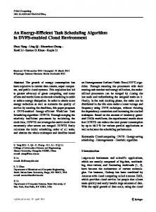
The following Table 1 and Table 2 list one of running results with MATLAB. In this simulation, there are 20 sensors node and 5 services and cycle time T=4. For each service s j , how many active sensors will be needed is given

and αiT .Table 1 and table 2 use the sleep mechanism in H2

section 3.1 and section 3.2 respectively.Figure.3 is the corresponding diagram of the energy consumption of every sensor node.

THE RESULT USED THE SLEEP MECHANISM IN SECTION 3.1

αitSL

p1

p2

p3

p4

p5

p6

p7

p8

p9

p10

p11

p12

p13

p14

p15

p16

p17

p18

p19

p20

t1 t2 t3 t4

1 1 1 1 4

0 1 1 0 2

1 1 1 1 4

0 1 1 1 3

1 0 1 1 3

0 1 1 0 2

1 0 1 1 3

0 1 0 1 2

1 0 1 0 2

0 1 1 1 3

1 0 1 1 3

1 1 1 1 4

1 1 1 1 4

0 1 1 1 3

0 1 0 0 1

0 1 1 1 3

0 0 0 1 1

0 0 0 1 1

1 1 1 1 4

1 1 0 1 3

EiL αH1

4

TABLE II.

THE RESULT USED THE SLEEP MECHANISM IN SECTION 3.2

αitSH

p1

p2

p3

p4

p5

p6

p7

p8

p9

p10

p11

p12

p13

p14

p15

p16

p17

p18

p19

p20

t1 t2 t3 t4

1 1 1 0 3

0 0 0 0 0

1 1 0 0 2

0 1 1 1 3

1 0 1 1 3

0 1 1 0 2

1 0 1 1 3

0 0 0 0 0

1 0 1 0 2

0 0 1 1 2

1 0 1 1 3

1 1 0 0 2

0 1 1 1 3

0 0 0 0 0

0 0 0 0 0

0 1 1 1 3

0 0 0 0 0

0 0 0 0 0

1 1 0 1 3

1 1 0 1 3

EiH αH 2

3

Figure 3. The comparison of energy consumption between Nodes Round Robin and Improved Sensor Nodes Round Robin

Published by Atlantis Press, Paris, France. © the authors 0074

Proceedings of the 2012 2nd International Conference on Computer and Information Application (ICCIA 2012)

Through comparing table 1 and table 2, we can clearly SH SL see that α H 2 ≤ α H 1 , because α it = 1 only when α it = 1 . We can obtain that the sleep mechanism in section 3.2 excels the sleep mechanism in section 3.1. At the same time, from the Figure 2, we can see that every sensor node’s energy consumption adopting the improved sensor node robin is less than or equal to the energy consumption adopting the sensor node robin. ACKNOWLEDGMENT The paper is supported by the Natural Science Foundation of China (NSFC) with Grant No. 60972004, and Nature Science Foundation of Beijing with Grant No. 4122073. REFERENCES [1] Peter Wolfs, Syed Isalm, “Potential Barriers to Smart Grid Technology in Australia”, Power Engineering Conference, pp.1-6, 2009. [2] Gopalakrishnan lyer, prathima Agrawal, “Smart Power Grids", 42nd South Eastern Symposium on System Theory, USA, 2010.

[3] Vehbi C.Gungor, Bin Lu, “Opportunities and Challenges of Wireless Sensor Networks In Smart Grid”, IEEE Transactions on Industrial Electronics, Vol. 57, no. 10, pp. 3557 – 3564,2010. [4] Wang yangguang, Yin xinggen, “Application of Wireless Sensor Networks in Smart Grid”, Power System Technology, vol. 34, no. 5, pp.7-11, 2010. [5] Tian D, Georganas N D, “A coverage-preserving node scheduling scheme for large wireless sensor networks”, In First ACM International Workshop on Wireless Sensor Networks and Applications. [6] Deng J, Han Y S, “Balanced-energy sleep scheduling scheme for high density cluster-based sensor networks”, Applications and Services in Wireless Networks, pp.99-108, 2004. [7] Liu Hai, Wan Peng-jun, “Maximal Lifetime Scheduling in Sensor Surveillance Networks”, Conference of the IEEE Computer and Communications Societies, vol. 4,pp.2482-2491, 2005. [8] Liu Jin-xia, “Research on Node Scheduling Schemes in Wireless Sensor Networks”, University of Science and Technology of China, China, 2009. [9] M. Ismail, M.Y.Sanavullah, “security topology in wireless sensor networks with routing optimisation”, Fourth International Conference on Wireless Communication and Sensor Networks, pp.1-15,2008. [10] Wang Jian-ping, Li De-ying, “Cross-Layer Sleep Scheduling Design in Service-Oriented Wireless Sensor Networks”. IEEETRANSACTIONSONMOBILE COMPUTING, VOL 9, NO 11, pp.1622-1633,2010

Published by Atlantis Press, Paris, France. © the authors 0075