An Efficient Unified Approach for the Numerical Solution of Delay

An Efficient Unified Approach for the Numerical Solution of Delay Differential Equations Hossein ZivariPiran and Wayne Enright Department of Computer Science, University of Toronto Toronto, ON, M5S 3G4, Canada {hzp, enright}@cs.toronto.edu

Abstract In this paper we propose a new framework for designing a delay differential equation (DDE) solver which works with any supplied initial value problem (IVP) solver that is based on a standard step-by-step approach, such as Runge-Kutta or linear multi-step methods, and can provide dense output. This is done by treating a general DDE as a special example of a discontinuous IVP. Using this interpretation we develop an efficient technique to solve the resulting discontinuous IVP. We also give a more clear process for the numerical techniques used when solving the implicit equations that arise on a time step, such as when the underlying IVP solver is implicit or the delay vanishes. The new modular design for the resulting simulator we introduce, helps to accelerate the utilization of advances in the different components of an effective numerical method. Such components include the underlying discrete formula, the interpolant for dense output, the strategy for handling discontinuities and the iteration scheme for solving any implicit equations that arise.

1 Introduction Differential equations are one of the most frequently used tools for mathematical modeling in engineering and life sciences. Delay differential equations (DDEs) are a class of differential equations that have received considerable recent attention and been proven to model many real life problems, traditionally formulated as systems of ordinary differential equations (ODEs), more naturally and more accurately. Several DDE solvers have been implemented during the past twenty years, based on the extension or modification of traditional ODE techniques such as those based on Runge-Kutta or linear multi-step formulas ([2], [4], [9], [11], [17], [20], [21]). The implementations of these solvers are usually based on adapting an existing initial value problem (IVP) solver. These DDE solvers use the provision for dense output, which is a key component of most modern IVP solvers, as the base and add some strategies for handling discontinuities and vanishing delays. During this

1

process, special properties of the underlying IVP solvers are usually exploited to make the overall technique more efficient. There are some drawbacks associated with this approach for developing DDE solvers. First, it usually takes a long time for an IVP solver to be recognized and subsequently identified as a candidate for modification for use as a DDE solver. Therefore, it is difficult to have a timely investigation of the effectiveness of proposed new underlying formulas (used in IVP solvers), for DDEs. Second, when some or all added components of a DDE solver, such as stepsize selection strategy and discontinuity handling, rely on the underlying IVP formula, they need to be redeveloped and recoded for every new DDE solver. This results in a lot of redundancy during the analysis and the coding, since many concepts involved in developing these components are common. In this paper we propose a structure for a DDE solver which is independent of the underlying IVP solver, with the only interactions between the two being through a common interface. We consider a general step-by-step IVP solver that finds continuous numerical approximations to problems of the general form y′ (t) = f (t, y(t)), for t0 ≤ t ≤ tF y(t0 ) = y0 ,

(1)

where y and f are vector-valued functions. The resulting DDE solver that we develop can be applied to approximate the solution of a system of retarded delay differential equations (RDDE), y′ (t) = f (t, y(t), y(t − σ1 ), . . . , y(t − σν )), for t0 ≤ t ≤ tF y(t) = φ (t), for t ≤ t0

(2)

or a system of neutral delay differential equations (NDDE) y′ (t) = f (t, y(t), y(t − σ1 ), . . . , y(t − σν ), y′ (t − σν +1 ), . . . , y′ (t − σν +ω )), for t0 ≤ t ≤ tF

(3)

y(t) = φ (t), y (t) = φ (t), for t ≤ t0 ′

′

where φ , the history, is a vector-valued function and σi = σi (t, y(t)) ≥ 0, i = 1, 2, . . ., ν + ω , are scalar functions (which can in general be time and state dependent). There are two major complications that can cause numerical difficulties in conventional approaches for solving DDEs: First, discontinuities may occur in various derivatives of the solution. Second, a delay may vanish, i.e. σ → 0. When a delay vanishes, we call it a vanishing delay. The first difficulty is due to the presence of the delay terms. In general at the initial point, the right-hand derivative y′ (t0 )+ , evaluated using f , does not equal the left-hand derivative φ ′ (t0 )− . Furthermore, φ may have discontinuities. A discontinuity can therefore arise and propagate from both the initial time and the history function. In general, the order of a derivative discontinuity (when it is propagated) increases with t for RDDEs, but this is not the case for NDDEs. 2

The second complication is important because it may cause a DDE solver to fail by forcing it to choose a sequence of very small steps. In the remainder of this paper we first review the techniques used in the numerical solution of discontinuous IVPs and show that a general DDE can be treated as a special example of a discontinuous IVP. In Section 5 we develop the details of a DDE solver based on this view and also the required interface with an IVP solver. In Section 6 we report on some numerical experiments with a DDE solver developed using this approach.

2 Discontinuous IVPs and Hybrid Systems Hybrid systems are mathematical models that exhibit both discrete and continuous behavior over the time interval of interest. The continuous behavior of the model is usually described by one or more ODEs, DDEs, or differential-algebraic equations (DAEs). The discrete behavior, which occurs at particular points in time (events), includes phenomena such as nonsmooth forcing, switching of the vector field and jumps in the state. This is a new perspective, that can be compared with the traditional approach of formulating the model in terms of discontinuous vector fields. (For more information and discussion of hybrid systems arising in mathematical modeling see [1] or [8] and references therein.) Consider a simple case of a hybrid system described using two sets of differential equations and a switching function, ( f1 (t, y(t)), for g(t, y(t)) < 0 y′ (t) = (4) f2 (t, y(t)), for g(t, y(t)) ≥ 0 To simulate the system (4), one has to use an integration scheme along with a transition handler. The integration is usually done by a Runge-Kutta method or a linear multistep method. The transition handler is responsible for detecting events and locating switching points and changing the integration accordingly (transition). An important aspect of the transition handler is the correct detection of irregularities that may happen at a switching point, such as non-uniqueness or termination of the solution. Suppose that the integration of the hybrid system (4) has reached tn where we have yn ≈ y(tn ). The local solution zn (t) over [tn ,tn+1 ] is defined by ( f1 (t, zn (t)), for g(t, zn (t)) < 0 z′n (t) = f2 (t, zn (t)), for g(t, zn (t)) ≥ 0 (5) zn (tn ) = yn .

3

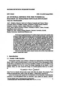
3 Techniques for the Efficient Simulation of Discontinuous IVPs Suppose that a solver is trying to compute a numerical approximation to the solution of (4) by computing a continuous approximation on each step. All standard solvers assume that the solution is continuous enough, over the entire step, for the underlying formulas to be applied with confidence. An accepted strategy is to detect and include the discontinuity points in the set of mesh points. For the successful application of this strategy, having an accurate discontinuity or switching point location is necessary. For a state-dependent switching function, the location of discontinuities cannot be computed a` priori because their unknown locations depend implicitly on the unknown solution. When the solver wants to take a step from tn to tn+1 , and a switching/discontiniuity is suspected to occur in [tn ,tn+1 ], approximations based on sufficient differentiability of the solution become unreliable. Therefore, using the local continuous approximation to the solution in [tn ,tn+1 ] to locate the discontinuity may lead to an inaccurate approximation (see Figure 1). A common treatment of this difficulty uses an iterative method which in turn computes the approximate solution y, and the zero crossing function of an associated event function g. Assuming that the iteration is convergent, the solution and the location of the discontinuity become more accurate on each iteration. The drawback of this method is the slow rate of convergence, which is linear in the best implementations. Here we give details of a more efficient treatment introduced by Ellison [5]. The idea is to somehow reduce the effect of locating the zero crossing of g on the computation of y. This can be done by defining the functions z[c] and g[c] as follows. z[c] is defined as the solution of (5) when we eliminate the effect of the switching point λ , by using a smooth extension of the local solution zn (t) after λ (see Figure 1), that is, z[c] is the solution of the local IVP, z′[c] (t) = fi (t, z[c] (t)), for tn ≤ t ≤ tn+1 z[c] (tn ) = yn ,

(6)

where the index i is determined using the state of the system (controlled by g) at tn and stays the same (either i = 1 or i = 2) for tn ≤ t ≤ tn+1 . Then, g[c] is defined as the switching (zero crossing) function computed using z[c] , g[c] (t) = g(t, z[c] (t)), (7) which is a function of only t, because z[c] (t) is defined as a usual IVP without any switching functions over [tn ,tn+1 ]. The governing systems of differential equations for zn (t) and z[c] (t) are the same before the switching point. Hence, we have, zn (t) = z[c] (t), for tn ≤ t < λ . 4

(8)

Then, it is not hard to see that, g[c] (t) = g(t, zn (t)), for tn ≤ t < λ .

(9)

Considering the limit case, lim g[c] (t) = lim g(t, zn (t)),

tրλ

tրλ

(10)

or (using the continuity of g[c] ), g[c] (λ ) = g(λ , lim zn (t)),

(11)

g[c] (λ ) = 0,

(12)

tրλ

which gives us, because λ is a switching point for zn (t). Equation (12) defines another function that crosses zero at λ . However, there is a big difference which makes Equation (12) very attractive. The difference is that g[c] is time dependent and also differentiable. This eliminates the possibility of computing a false solution (see Figure 1), and gives us a direct way of computing λ , by first computing z[c] and then applying a root finding algorithm to the associated g[c] . The differentiability of g[c] , which results from the differentiability of z[c] , enables us to apply efficient root finding methods such as Newton’s method or its variations. Standard numerical methods for IVPs compute an accurate approximation only for z[c] (tn+1 ). Therefore, an IVP method which provides an accurate continuous approximation is required for our root finding process. Those methods have been developed and are widely available. However, a numerical method used in practice only provides z¯[c] (t), an accurate approximation to z[c] (t) over [tn ,tn+1 ]. As a result, the function investigated by the root finder is actually g¯[c] (t) = g(t, z¯[c] (t)).

(13)

If g(t, y) is Lipschitz continuous and z¯[c] (t) ≅ z[c] (t), then any discrepancy between the computed roots of g¯[c] (t) and g[c] (t) will be within the accepted numerical error. A similar idea has been used by Park and Barton [14] for handling transitions in hybrid systems of differential algebraic equations.

4 DDEs as Discontinuous IVPs Consider a simple state-dependent retarded delay differential equation (RDDE) defined by y′ (t) = f (t, y(t), y(α (t, y(t)))), for t ≥ t0 y(t0 ) = y0 ,

(14)

y(t) = φ (t), for t < t0 5

y

true local solution false computed solution smooth extension of the solution discontinuity(switching) point

tn

λ

tn+1 t

g

t

Figure 1: A typical situation for a state-dependent switching function. The true local solution refers to the exact solution of Equation (5); the false computed solution refers to the continuous approximate solution of Equation (5) (produced by a standard IVP method); and smooth extension refers to z[c] (t) (Equation (6)). Different approximations to the switching function g are computed using the corresponding solution approximations and are identified accordingly.

6

where α (t, y(t)) = t − σ (t, y(t)), and f (t, y, v) is sufficiently differentiable with respect to t, y and v. With this assumption, the only discontinuities in the solution or its low order derivatives will be associated with the propagation of discontinuities introduced by the initial function or at the initial point. Now assume that jumps in one of the derivatives of y(t) with respect to t occur at the points (15) · · · < λ−2 < λ−1 < λ0 = t0 < λ1 < λ2 < · · · where λ j , j < 0, are discontinuities in the initial function. Then, artificial event functions gi (t, y(t)) = α (t, y(t)) − λi , i = . . . , −2, −1, 0, 1, 2, . . .

(16)

can be defined accordingly and used to write the equation characterizing the propagation of a discontinuity to λr , r ≥ 1,

λr = min{λ > λr−1 : λ is a root of odd multiplicity of gi (t, y(t)), i ≤ r −1}. (17) In other words, λr , r ≥ 1, is the leftmost discontinuity of all propagated discontinuities arising from {. . . , λ−1 , λ0 , λ1 , . . . , λr−1 } and lying in (λr−1 , +∞). The roots of gi (t, y(t)) with even multiplicity do not cause discontinuities and they do not need to be identified, since the delay argument, α (t, y(t)), crosses a previous discontinuity point only for roots which have odd multiplicity. Note that for the special case involving a single increasing delay argument and a smooth history function, φ (t); each discontinuity is caused by propagation from the most recent previous discontinuity point, namely,

α (λr , y(λr )) = λr−1 , r ≥ 1.

(18)

Using the explicit identification of all sources of non-smoothness, it is not hard to see that the solution of the system (14) also satisfies the following system of discontinuous IVPs, y′ (t) = fr (t, y(t)) = f (t, y(t), y[r] (α (t, y(t)))), for λr ≤ α (t, y(t)) < λr+1

(19)

y(t0 ) = y0 , where ( y(α ), for λr ≤ α < λr+1 y[r] (α ) = smooth extension from [λr , λr+1 ), for α < λr or α ≥ λr+1 .

(20)

The value of y[r] (α ) outside [λr , λr+1 ) is not required to be defined, as the right hand side of (19) switches if α goes outside this interval. Therefore, the smooth extension in (20) is only defined and used to facilitate the root-finding process during the numerical computations. 7

Now, using (16), Equation (19) can be rewritten in the standard form for discontinuous IVPs as y′ (t) = fr (t, y(t)), for gr (t, y(t)) ≥ 0 and gr+1 (t, y(t)) < 0

(21)

y(t0 ) = y0 . While (21) defines the switching functions, due to the (possible) presence of a C0 discontinuity (i.e. discontinuity in the value), the transition still needs to be clarified when there are different choices for the value at a discontinuity point. In a hybrid system, those discontinuities can come from jumps in the state which are triggered by specially defined events. Traditionally, due to the correspondence of systems with real phenomena, all C0 discontinuities are considered as transitions in state or control variables. Hence, the exact value of state or control variables at the point of discontinuity is not important, and can be considered to be evaluated using left or right segments. In this view, a discontinuity point is mainly considered as a border between two continuous segments. Therefore, if a value of a variable needs to be evaluated at a discontinuity point λ , the segment used for the evaluation is picked with respect to the underlying transition. This means that if λ is approached from left(right) and we need the value before the (possible) transition, then the left(right) segment is used, and if the value after the (possible) transition is needed then the right(left) segment is used.

5 Interfacing with IVP Integrators Assume that an approximate solution has been computed using a step-by-step IVP integrator over [t0 ,tn ] and now a step is to be taken from tn to tn+1 . If θ[r] (α ) is an associated accurate continuous approximation to y[r] (α ) (usually a piecewise polynomial), (21) can then be numerically integrated using the associated perturbed IVP, f (t, y(t), y[r] (α (t, y(t)))) ≅ f (t, y(t), θ[r] (α (t, y(t)))). (22)

5.1

Explicit IVP Integrators and Small/Vanishing Delays

Preserving explicit structure of the underlying IVP formula requires that the delay value, y(α ), be independent of the values introduced in the current step [tn ,tn+1 ]. The associated explicitness condition

α (t, y(t)) ≤ tn ,

∀t ∈ [tn ,tn+1 ],

can be monitored by introducing the local switching function, gne (t, y(t)) = α (t, y(t)) − tn ,

8

(where ‘e’ denotes “explicit”) and can be added to the system, (21), y′ (t) = fr (t, y(t)), for gr (t, y(t)) ≥ 0, gne (t, y(t)) ≤

gr+1 (t, y(t)) < 0,

0,

(23)

y(tn ) = yn . This formulation when combined with the approach for handling switching functions described in the previous section would impose the restriction that the stepsize tn+1 − tn be smaller than the minimum delay. In other words, if gne is triggered, say at te , then the current step is partitioned at te , and the next step starts at tn+1 = te . To avoid taking a series of extremely small steps in the case of a vanishing delay, we add a constraint, α (t, y(t)) < t − ε , where ε is a lower bound for small delays. The associated transition function is then, gv (t, y(t)) = α (t, y(t)) − t + ε , (24) and can be used to rewrite (23) as, y′ (t) = fr (t, y(t)), for gr (t, y(t)) ≥ 0, gne (t, y(t)) ≤

gr+1 (t, y(t)) < 0,

0,

(25)

gv (t, y(t)) < 0, y(tn ) = yn . If gv (t, y(t)) is triggered, continuing with the explicit integration is not numerically feasible as it will result in an excessive number of small steps. There are two possible strategies for resolving this difficulty: taking a few special steps with the explicit integrator to pass the vanishing neighborhood or temporarily switching to an implicit integrator. Here we describe a possible approach for taking the special steps. After gv (t, y(t)) is triggered, replace (23) with, y′ (t) = fr (t, y(t)) = f (t, y(t), θ[r] (α (t, y(t)))), for gr (t, y(t)) ≥ 0,

gr+1 (t, y(t)) < 0,

gv (t, y(t)) > 0,

(26)

y(tn ) = yn , where the component of θ[r] in [tn ,tn+1 ], which is needed during the current step, has not been computed yet. Considering the fact that this component can be approximated using the computed y, we observe a potential loop. A common approach to terminate this loop is to treat it as a system of nonlinear equations. For the numerical solution of the resulting system of nonlinear equations, fixed point 9

iterations or a modification of Newton-Raphson can be used. Here we give the details of fixed point iterations. (Note that this iteration is similar to the Picard iteration or the waveform relaxation iteration arising in the analysis of IVPs.) 1. Choose an initial guess for the interpolant Pn in [tn ,tn+1 ]. 2. Compute the solution using the interpolant Pn as a part of the history. 3. Update the interpolant Pn using the last computed solution. 4. If the sequence of updated interpolants has converged ⇒ stop. 5. Continue with (2). A good initial guess for the interpolant is usually obtained by extrapolation of the interpolant from the previous step. If there is not a previous step associated with the current step, or the previous step is not connected to the current step with sufficient continuity, then using extrapolation may not be possible or may give a poor result. In such cases an alternative is to treat the equations for the first iteration as specified below, y′ (t) = f˜(t, y(t)) = f (t, y(t), (1 − ξ )y(tn ) + ξ y(t)), for gr (t, y(t)) ≥ 0,

gr+1 (t, y(t)) < 0,

gv (t, y(t)) > 0,

(27)

y(tn ) = yn , where

ξ=

α (t, y(t)) − tn , t − tn

and then, after we compute y, use it to define the initial guess for Pn in [tn ,tn+1 ] and switch back to our original equations (26) for further iterations. The first order approximation (1 − ξ )y(tn ) + ξ y(t), usually leads to a more accurate starting approximation than the case when a constant approximation like y(tn ) is used. This formula can be justified using backward error analysis in form of the associated defect (assuming the Lipschitz continuity of f ) or, in other words, by observing that the residual after the first iteration will be at worse O(h2n ).

5.2

Implicit IVP Integrators

Since implicit integrators are usually used when the system of ODEs is stiff, taking large steps with these integrators is not unusual. Therefore, we may encounter the case with an unknown interpolant for the current step arises on a large fraction of the attempted steps. Furthermore, in this situation a vanishing delay need not be treated as a special case. We can consider the interpolant on the current step to be represented by the implicitly defined stages introduced on this step, and try to find it in a similar way that we solve for the discrete solution yn itself. Here we give 10

the details for Runge-Kutta (RK) methods and linear multistep methods (LMMs). Since RK methods and LMMs are special cases of general linear methods (GLMs), we use the standard formulation [3] for GLMs. The details for RK methods or LMMs can be derived by standard translations from GLMs (see [3] for details). The associated system of ODEs for [tn ,tn+1 ] is y′ (t) = fr (t, y(t)) = f (t, y(t), y[r] (α (t, y(t)))), for gr (t, y(t)) ≥ 0,

gr+1 (t, y(t)) < 0,

(28)

y(tn ) = yn . After defining the equations for the unknown stage values Y j , j = 1, . . . , s, a modification of Newton-Raphson is usually used to solve for these unknown vectors. This nonlinear iteration will involve the computations of Fj = fr (t j ,Y j ),

j = 1, 2, . . . , s

(29)

and

∂ Fj , ∂ Yk

j = 1, 2, . . . , s

(30)

k = 1, 2, . . . , s in an iterative scheme, attempting to converge to the solution of the nonlinear equations defining the unknown stage values. In the case of an unknown interpolant (α (t, y(t)) > tn for some t in [tn ,tn+1 ]), the theory of ODEs is not applicable directly. In the following we discuss a way to treat this case as a system of ODEs, even when an unknown interpolant is introduced. 5.2.1 Simultaneous Iterative Improvement Assume that Pn is the local polynomial interpolant (associated with the current step from tn to tn+1 ), which in the most general case has structural dependencies on [n] Y j , j = 1, 2, . . . , s and yi , i = 1, 2, . . . , q (input approximations), then ( independent of Y , for α < tn θ[r] (α ) = (31) Pn [Y, y[n] ](α ), for α ≥ tn [n]

[n]

[n]

where Y = {Y1 ,Y2 ,Y3 , . . . ,Ys } and y[n] = {y1 , y2 , . . . , yq } are used for convenience. In the following ( ∂∂Aq ) is used to indicate partial differentiation of a parametric multivariate function A w.r.t. a parameter or variable q, and ( dA dq ) is used to indicate the total derivative of such a function. Computing Fj : In either case of (31) the continuous approximation θ[r] (α ) is computable at all required points, provided that all components of Y are available. In our iterative improvement scheme, these values are determined from the latest iteration or are as the initial guess for the first iteration. 11

Computing

∂ Fj ∂ Yk

: Differentiating (29) and using (19) and (22),

∂ Fj ∂ f (t j ,Y j , θ[r] (α (t j ,Y j ))) × δ jk + = ∂ Yk ∂y d θ[r] (α (t j ,Y j )) ∂f (t j ,Y j , θ[r] (α (t j ,Y j ))) × , ∂v dYk

(32)

where δ jk denotes the Kronecker symbol. Using (31), d θ[r] (α (t j ,Y j )) = dYk ′ (α ) = where θ[r]

( ′ (α (t ,Y )) × ∂ α (t ,Y ) × δ , for α (t ,Y ) < t θ[r] j j j j n jk ∂y j j dPn [Y,y[n] ](α (t j ,Y j )) , dYk

d θ[r] (t) dt (α ),

for α (t j ,Y j ) ≥ tn (33)

and

dPn [Y, y[n] ](α (t j ,Y j )) ∂α (t j ,Y j ) × δ jk + = Pn′ [Y, y[n] ](α (t j ,Y j )) × dYk ∂y ∂ Pn [Y, y[n] ](α (t j ,Y j )) ∂ Yk (34) ∂α ′ = θ[r] (α (t j ,Y j )) × (t j ,Y j ) × δ jk + ∂y ∂ Pn [Y, y[n] ](α (t j ,Y j )), ∂ Yk where Pn′ [Y, y[n] ](α ) =

dPn [Y,y[n] ](t) (α ). dt

Combining (32), (33) and (34), ∂ Fj ∂f = (t j ,Y j , θ[r] (α [ j])) ∂ Yk ∂y ∂f ∂α ′ + (t j ,Y j , θ[r] (α [ j])) × θ[r] (α [ j]) × (t j ,Y j ) × δ jk + ∂v ∂y ( 0, for α [ j] < tn ∂f ∂ Pn [n] ∂ v (t j ,Y j , θ[r] (α [ j])) × ∂ Yk [Y, y ](α [ j]), for α [ j] ≥ tn

(35)

where α [ j] = α (t j ,Y j ). ∂F

The first component of ∂ Ykj in (35) has the same structure as that arising in the corresponding IVP problem, due to the presence of δ jk . For delays smaller than the step size, adding the second component of (35) results in a different structure for the Jacobian. For an efficient implementation, usually an approximation of this Jacobian is used. Therefore, one might ignore the second component completely, or replace it with something with the same structure (H δ jk , for any, but usually a heuristically chosen, matrix H). 12

At present, we do not know of any mathematical or numerical evidence that shows the safety of this replacement (i.e., not causing divergence of iterations during the solution process). The second term represents the numerical complexity inherited from the presence of delays in the model. We are currently seeking possible problems (i.e., stiff DDEs) that necessarily need this second component for the convergence of the iterations. We are also looking for techniques to incorporate this term efficiently in the computation process, while respecting a generic interface (to be designed) between the DDE solver and IVP solvers.

5.3

Neutral Problems

For a system of NDDEs (3), including a term y′ (t − σ ) or y′ (α ) as an argument of f , will lead to modifications to some of our expressions. Here, we discuss the important changes. In the vanishing delay case for explicit formulas, if the vanishing delay appears in a derivative term, the same process can be applied, with Pn′ playing a similar role for y′ (α ) as Pn did for y(α ). However, if we have to use Equation (27), we can use the approximation y′ (α (t, y(t))) ≈ y′ (tn ). In this case, y′ (tn ) should be provided as an external value. We do not consider the case of an NDDE with accumulated discontinuities at a vanishing delay, because such problems can be mathematically ill-posed. For delays appearing in derivatives, the second term in Equation (32) should be changed to ′ (α (t ,Y )) d θ[r] j j ∂f ′ (t j ,Y j , θ[r] , (α (t j ,Y j ))) × ∂w dYk where f = f (t, y, w), and also all instances of θ[r] and Pn should be replaced with ′ and P ′ , respectively, in the subsequent Equations (33, 34, 35). θ[r] n

5.4

Extension to Multiple Delays

For a general system of DDEs with multiple delays (2), one must define corresponding switching functions for each delay, separately. The implementation of an effective DDE method becomes much more complex, since we have to monitor multiple switching functions and find the first one that is triggered on each step. The equations for the implicit solver can then be derived by taking the sum over all delays α of the term, d θ[r] (α (t j ,Y j )) ∂f (t j ,Y j , θ[r] (α (t j ,Y j ))) × , ∂ vα dYk appearing in (32). 13

6 Numerical Experiments Based on the ideas presented here, we have developed an experimental code DDEM. The code is currently able to use any explicit step-by-step IVP solver, which provides an accurate local interpolant. For our experiments we use the IVP method CRK6X, which is an order 6 explicit continuous Runge-Kutta method with defect control (developed and discussed in [6]).

6.1

Test Problems

The following problems are used to test the effectiveness of the proposed methods. “Test Problem 1” and “Test Problem 3” have state-dependent delays and were chosen to test the discontinuity tracking strategy of our method. “Test Problem 2” is an NDDE with many discontinuities and is used to test efficiency of the solver when dealing with persisting discontinuities and also to show its applicability for systems of DDEs. “Test Problem 4” and “Test Problem 5” have vanishing delays, during the integration and at the starting point, respectively. They were chosen to test the iterative scheme for handling vanishing delays. “Test Problem 6” is a 4-dimensional problem with two constant delays. For DDEM, we have considered this problem a vanishing delay problem by setting the lower bound constant in Equation (24) to be a value bigger than the smallest constant delay; otherwise forcing the explicitness condition will require at least (tF − t0 )/(the smallest delay) = (350 − 0)/0.15 ≈ 2333 steps. All these problems are nonstiff. Test Problem 1 [16]: y′ = y(y(t)), for t in [2, 5.5]. The history function is y = 0.5, for t < 2 and y(2) = 1. The C0 discontinuity of the solution at ξ0 = 2 introduces break points at ξ1 = 4 (C1 ) and ξ2 = 4 + 2 ln 2 ≈ 5.386 (C2 ). The exact solution to this problem is   t/2, 2 exp(t/2 − 2), y(t) =  4 − 2 ln(1 + ξ2 − t)

for ξ0 ≤ t ≤ ξ1 for ξ1 ≤ t ≤ ξ2 for ξ2 ≤ t ≤ 5.5

Test Problem 2. A neutral delay logistic Gause-type predator-prey system [12]:

14

y2 (t)y1 (t)2 y′1 (t) = y1 (t)(1 − y1 (t − τ ) − ρ y′1 (t − τ )) − , y1 (t)2 + 1 y1 (t)2 y′2 (t) = y2 (t) −α , y1 (t)2 + 1 where α = 1/10, ρ = 29/10 and τ = 21/50, for t in [0, 30]. The history functions are 1 33 − t, 100 10 1 111 + t, φ2 (t) = 50 10

φ1 (t) =

for t ≤ 0. The solution is C1 discontinuous at the starting point which propagates as C1 and C2 discontinuities to y1 (t) and y2 (t), respectively, at t = nτ for n ≥ 1. The exact solution of this problem is unknown. Test Problem 3 [13]: y(t)y(ln(y(t))) , t for t in [1, 10]. The history function is y′ (t) =

φ (t) = 1 for t ≤ 1. The exact solution to this problem is  t,     exp(t/e), e y(t) = e ,   3−ln(t)   not known,

for 1 ≤ t ≤ e for e ≤ t ≤ e2 for e2 ≤ t ≤ e3 for e3 < t

where e3 = exp(3 − exp(1 − e)). Derivative jump discontinuities occur at t = 1 (C1 ), t = e (C2 ), t = e2 (C3 ) and t = e3 (C4 ).

Test Problem 4 [15]: y′ (t) = y(t − t −10 ), for t in [1, 10]. The history function is

φ (t) = t for t ≤ 1. The exact solution of this problem is unknown. This DDE has a vanishing (but non-singular) lag (limt→+∞ t −10 = 0; however, depending on the precision used, the vanishing behavior will first be recognized at some finite time t ⋆ and persists for all t > t ⋆ ). 15

Test Problem 5 [19]: y′ (t) = y(y(t)) + (3 + µ )t (2+µ ) − t (3+µ ) , 2

for t in [0, 1]. The initial value is y(0) = 0. The exact solution to this problem is y(t) = t (3+µ ) for 0 ≤ t ≤ 1. This is an initial value DDE with no discontinuities. We use µ = 0 in our experiments. The exact solution is a low degree polynomial and any IVP method should have no trouble with this problem. Test Problem 6. The SEIR epidemic model of Genik & van den Driessche [7]: −d τ , S′ = A − dS(t) − λ S(t)I(t) N(t) + γ I(t − τ )e

S(t−ω )I(t−ω ) −d ω E ′ = λ S(t)I(t) e − dE(t), N(t) − λ N(t−ω )

ω )I(t−ω ) −d ω − (γ + ε + d)I(t), e I ′ = λ S(t−N(t− ω) ′ −d R = γ I(t) − γ I(t − τ )e τ − dR(t),

where N(t) = S(t) + E(t) + I(t) + R(t), and A = 0.33, d = 0.006, λ = 0.308, γ = 0.04, ε = 0.06, τ = 42, ω = 0.15, for t in [0, 350]. The history functions are S = 15, E = 0, I = 2, R = 3, for t ≤ 0. The exact solution of this problem is unknown.

6.2

Results

Here we present the numerical results for the chosen test problems. We include results for a new version [10] of RADAR5 (Guglielmi and Hairer [9]), and DDE SOLVER (Thompson and Shampine [20]). We have set all absolute tolerances and the relative tolerance to TOL with TOL=10−6 ,10−9 for all solvers. The analytic solution or a very accurate approximation of it, obtained with a very small tolerance (TOL = 10−11 ), was used for computing the reported endpoint accuracy. The statistics we report in the tables are : 16

Table 1: Summary Statistics for Problems 1 to 6 (TOL = 10−6 ).

PROBLEM

SOLVER

STEPS

REJECTS

FCN

ABS ERR

REL ERR

1

DDE SOLVER RADAR5 DDEM

15 13 7

6 4 0

198 120 80

1.0 · 10−11 3.1 · 10−8 1.4 · 10−7

2.5 · 10−12 7.4 · 10−9 3.4 · 10−8

2


907 369 135

947 130 23

16884 4592 1810

1.4 · 10−7 8.6 · 10−8 6.5 · 10−7

4.4 · 10−7 8.8 · 10−8 7.4 · 10−7

3


31 28 18

12 1 2

405 225 223

9.9 · 10−8 1.0 · 10−5 9.0 · 10−6

2.4 · 10−9 2.7 · 10−7 2.2 · 10−7

4


118 73 64

10 1 4

2673 608 792

9.4 · 10−3 7.8 · 10−3 7.7 · 10−4

1.2 · 10−6 1.0 · 10−6 1.0 · 10−7

5


13 4 12

0 0 3

153 29 172

1.1 · 10−9 0.0 2.0 · 10−7

1.1 · 10−9 0.0 2.0 · 10−7

6


211 119 417

12 1 0

4923 1413 4836

6.8 · 10−8 6.7 · 10−7 1.6 · 10−8

5.8 · 10−7 5.2 · 10−6 2.9 · 10−7

STEPS: The number of successful steps. REJECTS: The number of rejected steps. FCN: The total number of derivative evaluations. ABS ERR: The global absolute error at the end point of integration (maximum over all components for multidimensional problems). REL ERR: The global component-wise relative error at the end point of integration (maximum over all components for multidimensional problems).

17

Table 2: Summary Statistics for Problems 1 to 6 (TOL = 10−9 ).

PROBLEM

SOLVER

STEPS

REJECTS

FCN

ABS ERR

REL ERR

1


21 24 12

11 5 3

297 207 168

6.6 · 10−12 5.6 · 10−9 2.1 · 10−9

1.5 · 10−12 1.3 · 10−9 4.9 · 10−10

2


1718 918 376

1577 123 150

29655 10063 5858

9.5 · 10−11 3.8 · 10−10 6.3 · 10−10

4.4 · 10−11 1.1 · 10−9 2.8 · 10−10

3


68 70 47

18 1 3

792 525 553

1.4 · 10−10 1.0 · 10−7 1.5 · 10−8

3.6 · 10−12 2.6 · 10−9 3.7 · 10−10

4


789 201 144

18 2 6

15453 1672 1735

3.5 · 10−5 1.1 · 10−5 4.9 · 10−6

4.5 · 10−9 1.5 · 10−9 6.7 · 10−10

5


16 4 23

6 0 6

243 29 325

3.2 · 10−11 0.0 3.3 · 10−10

3.2 · 10−11 0.0 3.3 · 10−10

6


447 281 480

14 10 6

9360 3146 5627

3.7 · 10−11 3.5 · 10−9 2.1 · 10−9

2.5 · 10−11 6.4 · 10−8 3.8 · 10−8

18

6.3

Discussions and Conclusions

The numerical results clearly show that for these particular examples, the derived DDE solver is competitive with a state of the art special purpose DDE solver. These results are chosen from a more extensive investigation that we have performed on different problems using standard DDE test sets [18], and confirm our claim that the generality we have introduced does not cause a noticeable inefficiency compared to specially designed DDE solvers. We are currently working on the details of the interface for implicit solvers and hope to find a design that preserves this property. The code DDEM and several driver programs are available at the address ‘http://www.cs.toronto.edu/∼hzp’.

References [1] Barton, P.I. and Pantelides, C.C.: Modeling of combined discrete/continuous processes. AIChE J., 40(6), 966-979 (1994) [2] Bocharov, G.A. and Marchuk, G.I. and Romanyukha, A.A.: Numerical solution by LMMs of stiff delay differential systems modelling an immune response, Numer. Math., 73, 131–148 (1996) [3] Butcher, J.C.: Numerical Methods for Ordinary Differential Equations, 2nd Edition, J. Wiley, Chichester, (2008) [4] Corwin, S. C. and Sarafyan, D. and Thompson, S.: DKLAG6: a code based on Continuous imbedded sixth-order Runge-Kutta methods for the solution of state-dependent functional differential equations, Appl. Numer. Math., 24, 319– 330 (1997) [5] Ellison, D.: Efficient Automatic Integration of Ordinary Differential Equations with Discontinuities, Math. Comput. Simut., 23(1), 12–20 (1981) [6] Enright, W.H. and Yan L.: The Quality/Cost Trade-off for a Class of ODE Solvers, Numerical Algorithms, DOI 10.1007/s11075-009-9288-x, (2009) [7] Genik, L. and Van Den Driessche P.: An Epidemic Model with RecruitmentDeath Demographics and Discrete Delays. In: Ruan, S., Wolkowicz, G.S.K. and Wu, J. (eds.) Differential Equations with Applications to Biology, Fields Institute Communications, No. 21, 237–249, American Mathematical Society, Providence, RI, (1999) [8] Grossman, R.L., Nerode, A., Ravn, A.P., and Rischel, H.: Hybrid Systems. Lecture Notes in Computer Science, Vol. 736, Springer-Verlag, New York, (1993) [9] Guglielmi, N. and Hairer, E.: Implementing Radau II-A methods for stiff delay differential equations, Computing, 67, 1–12 (2001) 19

[10] Guglielmi, N. and Hairer, E.: Computing breaking points in implicit delay differential equations, Advances in Computational Mathematics, 29(3), 229– 247 (2008) [11] Hayashi, H.: Numerical solution of retarded and neutral delay differential equations using continuous Runge-Kutta methods, PhD Thesis, Department of Computer Science, University of Toronto, Toronto, Canada, (1996) [12] Kuang, Y.: On Neutral Delay Logistic Gause-Type Predator-Prey Systems, Dynamics and Stability of Systems, 6, 173–189 (1991) [13] Neves, K.W.: Automatic Integration of Functional Differential Equations: An Approach, ACM Trans. Math. Soft., 1(4), 357–368 (1975) [14] Park, T. and Barton, P.: State Event Location in Differential Algebraic Models, ACM Transactions on Modeling and Computer Simulation, 6(2), 137–165 (1996) [15] Paul, C.A.H.: Runge-Kutta Methods for Functional Differential Equations, PhD. Thesis. University of Manchester (1992) [16] Paul, C.A.H.: Developing a Delay Differential Equation Solver, Appl. Numer. Math., 9, 403–414 (1992) [17] Paul, C.A.H.: A user-guide to Archi: An explicit Runge-Kutta code for solving delay and neutral differential equations and Parameter Estimation Problems, Technical Report, Department of Mathematics, University of Manchester, Manchester, England, 283, (1997) [18] Paul C.A.H.: A Test Set of Functional Differential Equations, Numerical Analysis Report, Manchester Centre for Computational Mathematics, Manchester, England, No. 243, (1994) [19] Tavernini, L.: The Approximate Solution of Volterra Differential Systems with State-Dependent Time Lags, SIAM J. Numer. Anal., 15 (5), 1039–1052, (1978) [20] Thompson, S. and Shampine, L.F.: A Friendly Fortran DDE Solver, Appl. Numer. Math., 53(3), 503–516 (2006) [21] Will´e, D.R. and Baker, C.T.H.: DELSOL - A Numerical Code for The Solution of Systems of Delay-Differential Equations, Appl. Numer. Math., 9, 223– 234 (1992)

20