{schakraborty,mpaul}@csu.edu.au, Charles Sturt University. *. {Manzur.murshed ... provides better rate distortion performance by exploiting coding efficiency in ... the highly accepted Mixture of Gaussian (MoG)-based dynamic background ...
AN EFFICIENT VIDEO CODING TECHNIQUE USING A NOVEL NONPARAMETRIC BACKGROUND MODEL Subrata Chakraborty*, Manoranjan Paul*, Manzur Murshed+, and Mortuza Ali+ * {schakraborty,mpaul}@csu.edu.au, Charles Sturt University * {Manzur.murshed,Mortuza.ali}@federation.edu.au, Federation University Australia ABSTRACT Video coding technique with a background frame, extracted from mixture of Gaussian (MoG) based background modeling, provides better rate distortion performance by exploiting coding efficiency in uncovered background areas compared to the latest video coding standard. However, it suffers from high computation time, low coding efficiency for dynamic videos, and prior knowledge requirement of video content. In this paper, we present a novel adaptive weighted non-parametric (WNP) background modeling technique and successfully embed it into HEVC video coding standard. Being non-parametric (NP), the proposed technique naturally exhibits superior performance in dynamic background scenarios compared to MoG-based technique without a priori knowledge of video data distribution. In addition, the WNP technique significantly reduces noise-related drawbacks of existing NP techniques to provide better quality video coding with much lower computation time as demonstrated through extensive comparative studies against NP, MoG and HEVC techniques. Index Terms—Video coding, Background model, Nonparametric model, Coding efficiency, Coding performance 1. INTRODUCTION Providing better quality video at a lower bit rate is the unsolved age old conquest for researchers in video coding domain. The key to solving this challenge is to strike the right balance to provide the best possible quality for the available bit rate. With the advancement of technology and the availability of high speed networks, larger bandwidths currently exist. However, sophisticated video capturing, display technologies, and incremental users’ demand on higher resolution and quality also produce large sized video data. Hence the challenge to find the appropriate balance between quality and bit rate still remains. The latest HEVC video coding standard [1] improved the coding performance by applying a number of innovative tools compared to its predecessor H.264/AVC [2] including a wider range of variable block size motion estimation (ME), motion compensation (MC), prediction, and transformation units. The use of multiple reference frames (MRFs) using variable block sizes tools typically provides better coding performance than single reference frame approach [1]-[3]. Some fast coding techniques [4][7] achieved significant time saving compared to H264 but failed to outperform it in rate-distortion (RD) coding performance for video with repetitive motion, uncovered background, non-integer pixel displacement, lighting change, etc. [8]. The image quality degradation and fluctuation problems related to the use of I-frames are well-known issues of the H264 standard [9]-[11] and studies
were conducted to find better I-frame selection process and use it as a second reference frame to overcome RD performance problem by the fast coding techniques and existing quality fluctuation problems [12]. Video segmentation based coding techniques tried to exploit the stable parts in a frame by treating them as background [13][15]; however they are highly computation intensive. Object segmentation based sprite coding techniques [16][17] were also introduced but they suffer from high computation burden and their performance degrades at high bit rate [18]. A number of video coding schemes using McFIS (most common frame in scene) [8][12][19][20] were introduced to utilize the highly accepted Mixture of Gaussian (MoG)-based dynamic background modeling (DBM) techniques [21][22]. The coding schemes using the McFIS further instilled the fact that using a good quality background frame as a reference frame improves coding performance and computational efficiency for static and uncovered background areas compared to the coding scheme with MRFs using a number of previously decoded frames. It also established the need for using a good DBM technique for practical usage. Studies show the improved performance and computational efficiency of the McFIS-based video coding schemes [8][12][19][20][23]. DBM is also applied in recent studies in the area of transcoding technique for video surveillance [24]. MoG based DBM works at pixel level where each pixel of a scene is modeled independently using a mixture of Ψ (generally 3 to 5) Gaussian distributions [21]-[23][25][26]. Although the MoG based DBM techniques have been proved successful and widely used by researchers and practitioners, they require the user to assume the data distribution in advance and relevant parameters must be set based on this underlying assumption. It is also found to be performing poorly for fast changing background environments [25][27]. A relatively new non-parametric (NP) techniques [25][27][28] has gained the attention of many researchers due to its ability to perform well in highly dynamic scenarios and it requires no initial assumption about the underlying data distribution[25][27][29]. The NP technique uses historical pixel values for a given pixel to perform probability density estimation using kernel estimator K where the kernel width is estimated considering two sources of variations – (i) edge of different objects passing through a pixel at different times giving large scale pixel fluctuations, and (ii) local intensity variation due to blurring of image [25][27]. The background model for a frame is developed by comparing the probability of the current intensity value of each pixel against a threshold (to decide whether background or foreground). The probability estimation is done based on the pixel’s historical values in the previous frames by calculating the
median of absolute pixel intensity differences between the current frame and each of the previous frames [25][27]. Although the high sensitivity to dynamic background environment makes the NP technique very attractive for applications such as object detection and tracking, this poses a serious challenge for video coding. If the background is updated more frequently then coding of more background frames would be necessary. This leads to a higher bit rate requirement. Moreover, in the existing NP technique [25][27], the background is generated using the pixel intensity values of the last frame only and the historical pixel intensity values are only used for probability estimation purpose. Hence, the background is heavily biased to the last frame and loses the historical trend value. This might provide a good background frame for detecting an object for the current frame for object detection applications; however, as an extra reference frame, it does not contribute significantly in video compression of the current frame as the last frame has normally been used for ME and MC of the current frame in HEVC or H.264. To resolve these issues we propose a novel weighted nonparametric (WNP) technique where we generate a more stable background using historical pixel values and the latest pixel value of the latest frame. The new technique uses the weighted average of (i) a probabilistic pixel intensity value (calculated based on median of historical values and randomly scaled standard deviation) and (ii) the latest pixel intensity value. This process scales the actual pixel intensity value by maintaining the historical trend of the intensities of the pixel position in the generated background. The background remains more stable, thus reducing the frequent background updating issue with NP. The new WNP technique inherits the advantages of the NP technique such as capacity to detect dynamic background better and ability to perform probability estimation with dynamic data distribution. The additional ability of WNP to provide a more stable background makes it more suitable for video compression purpose as it reduces the computational time significantly and provides better RD coding performance. The proposed DBM scheme captures more background areas compared to existing one so that we do not need to use ME for those areas and eventually it saves valuable computational time. In the following sections we first present the proposed WNP technique followed by detailed experimental results and discussions of the new technique. 2. PROPOSED TECHNIQUE The MRFs technique facilitates better predictions than using a single reference frame, targeting at video with features such as repetitive motion, uncovered background, non-integer pixel displacement, lighting change, etc. To reduce computational time associated with MRFs, a number of techniques [30][31] use dual reference frames: a long term reference (LTR) frame and a short term reference (STR) frame. The basic assumption of the dual reference frames for encoding the current frame is that the STR would be referenced for local motion i.e., moving areas, and the LTR would be referenced for still regions i.e., background areas of the frame. Our proposed technique presented in this study uses dual reference frames technique where the LTR is a high quality background frame (generated by the proposed WNP background modeling) and the STR is the immediate previous frame of the current frame. The background frame is modeled with a small number of original frames of a scene and encoded at high quality as a LTR frame. All frames in the scene are encoded using dual
reference frames. The Lagrangian RD cost function of the HEVC is used to finally select the reference frame for a block or subblock. We also incorporate a scene change detection strategy similar to [12]. When a scene change occurs we reset the background modeling and generate a new background frame for the new scene. To reduce the computational time, we use small search range for ME when we use the LTR frame (i.e., the background frame) as reference in the proposed scheme. As the LTR frame is referenced mainly for static and uncovered areas, we do not need to use larger search range. Thus, we can reduce the computational time significantly compared to existing dual reference frames-based techniques. The proposed WNP technique is primarily based on the wellknown NP Technique [25][27][28]. The WNP aims to generate a stable background frame from a set of initial training frames. The generated background frame integrates both historical pixel intensity value and recent pixel intensity value from the last training frame for each pixel. This retains the past pixel intensity trend as well as the recent pixel value which in turn will provide a more stable background for video compression purpose. The use of historical pixel values also eliminates a sudden pixel intensity change (i.e., noise or dynamic background impulse) of the latest frame compared to the historical trend. For object detection applications, considering the pixel intensity of the latest frame to generate background frame as done in NP technique provides better object in dynamic background situation. However, considering combination between the pixel intensity of the latest frame and the historical pixel value provides better RD performance in video coding applications (see the RD performance in Fig. 1). Note that the main objective of the video coding applications using background modeling is to reduce the residual error for improving compression performance whereas the main objective of the object detection applications is to find the object in its original shape. Thus, proposed background frame comprising historical pixel intensities ensures overall minimization of residual error of all frames, resulting in better overall compression. The proposed background modeling and background generation method can be described in the following 2 steps: Step 1: Background probability estimation technique ([25][27][28]) Given x1 , x2 ,..., x N is a set of recent intensity values for a pixel. We can estimate the probability density function with pixel intensity xt at time t by using the kernel estimator K(.) as p r ( xt )
1 N
N
K ( xt xi )
(1)
i 1
where K(.) is a kernel estimation function. If we consider that the kernel estimator function K(.) to be a Normal function N (0, ) where is the kernel function bandwidth, then the density estimation can be determined as
pr ( xt )
1 N
N
1
d i 1 (2 ) 2
1 2
e
1 ( xt xi )T 1 ( xt xi ) 2
(2)
With the assumption of independence between the different color channels d and with different kernel bandwidths 2j for the jth color channel we can write
12 0 0 2 0 2 0 . 0 32 0
suggest that finding the right balance between historical and recent pixel value is the key to selecting an appropriate value. In order to select the value we have developed an adaptive procedure described in 6 stages:
1) Decide the potential values
The density estimation equation then can be reduced to 1 p r ( xt ) N
N
d
i 1 j 1
1 2 2j
e
At
2 1 ( xt j xi j )
2
2j
(3)
In order to estimate the kernel bandwidth 2j for j-th color channel for any given pixel we need to compute the median absolute deviation over the sample for consecutive intensity values of the pixel. The median difference m can be calculated as m median (| xi xi 1 |) where i 1,2,..., N 1
We can consider that the intensity pair being consecutive comes from local-in-time distribution. Assuming that the local-intime distribution is Normal N ( , 2 ) , then the deviation ( xi xi 1 ) is also Normal N (0,2 2 ). The standard deviation of the first distribution can be computed as
m /(0.68 2 )
(4)
The synthesized value M is a mimic of the actual pixel intensity generated using the standard deviation and a very small normally distributed random multiplier Y which can generated using the randn(.) function in Matlab which generates a normally distributed random value. This is then used to generate the synthesised pixel value considering the calculated median as mean and using the calculated standard deviation . The value X of the background pixel can be calculated as a weighted average of the actual value xt and synthesized value M: X xt M (1 )
stage
we
decide
a
set
of
potential
for a given video dataset. The values are between 0 and 1 and may be selected at regular intervals.
2) Generate background for each
A background frame is generated for each by applying the background generation method described earlier. We can denote the backgrounds as B p where p 1...P.
3) Calculate pixel intensity variation
With the assumption of Fq where q 1...Q
training frames
with width W and height H, we find the intensity difference I for each pixel of each frame with the corresponding pixel for each background can be calculated as: I pq ( w, h) | B p ( w, h) Fq ( w, h) |
(6)
where p 1...P; q 1...Q; w 1...W ; h 1...H
Step 2: Background generation With the NP technique, the calculated pr ( xt ) is compared against a threshold of 20% variation to determine if the current pixel belongs to background or foreground. If the pixel is considered as background then its value is retained in the background frame. In the proposed WNP technique we also determine the background using a 20% variation threshold recommended in [27]. Once the current pixel value xt is detected as background, the value is combined with the synthesized historical pixel intensity of the given sample for that particular pixel. The synthesized historical pixel value M for the sample pixel values can be calculated as M median ( x1 , x 2 ,..., x N ) * Y
this
p where p 1...P is the number of values we are interested in
(5)
In this way, a background frame is generated for entire frame and then encoded with high quality. Corresponding quantization set up is similar to [12]. Selecting : The value of can be adaptively adjusted to provide more importance to either the recent value or the historical value trend for a given pixel. We have conducted simulation studies which show that the impact of is dependent on the video dataset. Please note that when we use 1 in the proposed method, the proposed method is equivalent to the traditional NP technique as the background is developed solely based on the most recent pixel value (see (5)). Our studies with other video data sets
4) Count background pixel detection The background detection percentage represents the area of a frame detected as background by the new WNP method using a particular value. The total number of pixels in a frame is W * H . The number of pixels detected as background in a frame using a particular value can be calculated applying (6) as C pq Count ( I pq ( w, h) )
(7)
The small value is the threshold for a pixel to be considered as background. Ideally, the value of should be “0”. However the WNP develops a synthesized background using historical and actual pixel values which leads to deviation from the actual pixel value and thus a nonzero value for some cases. With a significant amount of experimental studies using test videos we have identified that generally a large change in the pixel value classifies it as foreground pixel, while only a small change classifies it as background pixel. Experimental results indicate that up to 2% deviation from the highest possible pixel value (i.e. 255) may be used as the value.
5) Calculate background detection percentage By applying (7) we can calculate the percentage of total pixels detected as background for a particular frame by: U pq (C pq *100) /(W * H )
(8)
The overall background detection percentage for a test video is calculated based on the number of training frames Fq . The overall background detection percentage for the set p can be calculated as: Q
U p ( U pq ) / Q q 1
(9)
6) Select for a video The value for a given video is p for the maximum U p value.
p for max(U p ) where p 1,2,...P
(10)
Our experimental results show that the value that helps detecting the maximum percentage of background provides a better background reference frame for that video leading to better coding performance. The values were found to be positively correlated with the coding performance of any test video. This objective and adaptive selection procedure for the value provides the decoder with the ability to generate the best background to achieve best possible coding quality. 3. EXPERIMENTAL RESULTS & DISCUSSIONS 3.1. Experiment Setup The experiments were conducted on a dedicated desktop machine (with Intel core i7 3770 CPU @ 3.4 GHz, 16GB RAM and 1TB HDD) running 64 bit Windows operating system. The program codes for the NP technique were available from the author
Fig. 1 shows the RD performance for three test video sequences highlighting the significantly improved performances of the proposed WNP technique against other exisitng techniques. Detail results for our test video sequences are presented in Table 1. We observed that our proposed WNP technique provides significant PSNR gains over other techniques tested. For the Sales video sequence WNP achieves PSNR gains of 1dB, 0.9dB and 1.2dB to 3.1dB compared to NP, MoG and HEVC respectively. For the Silent video sequence the PSNR gains of the proposed WNP are 0.9dB to 1.1dB, 0.85dB to 1.1dB and 2dB to 2.6dB against NP, MoG and HEVC respectively. For the Gramdma video sequence WNP showed a PSNR gain of 1dB, 1dB to 1.05dB and 1.2 dB to 1.95dB compared to NP, MoG and HEVC respectively. For the Paris video sequence WNP PSNR gains were recorded as 0.4dB to 0.8dB, 0.45dB to 0.8dB and 1dB to 1.6dB compared to NP, MoG and HEVC respectively. For the Container video sequence WNP achieved PSNR gains of 0.6dB to 0.7dB, 0.6dB to 0.7dB and 0.65dB to 0.7dB against NP, MoG and HEVC respectively. The News video sequence is particularly challenging as the background contains very dynamic changes. For this sequence WNP registered PSNR gains of 0.1dB to 0.5dB, 0.2dB to 0.45dB and 0.9dB to 1.6dB compared to NP, MoG and HEVC respectively. The Table
(a) Result for Grandma Video (b) Result for Silent Video (c) Fig. 1: Coding quality performance of various methods for different standard video.
[25][27]. Each test video has been coded-decoded using the HEVC, NP, MoG [26] and WNP based coder-decoder. For HEVC we used GOP of size 30. For Inter coding we used 2 reference frames. Motion search was performed within a window of ±31. For NP, MoG and WNP, the generated background frame by each technique was used as a reference frame along with the immediate previous frame for coding-decoding purpose. The test video sequences Sales, News, Grandma and Table Tennis are of resolution of 176 × 144, while the Silent, Paris and Container test video sequences are of resolution of 352 × 288. First 25 frames were used as training frames of a scene to generate the background frame for the MoG, NP and WNP techniques. The initial total training frames were chosen 25 because it will provide a buffering time of < 1 second at standard 30fps. This is acceptable for the most of the applications. Also a set of 25 frames was large enough size to provide a good quality background for all our test video sequences. However, this size can be adjusted according to available buffering time and required background quality. We have used 5 different quantization values (QP=28, 24, 20, 16, and 12) for each sequence to obtain different bit rates and corresponding PSNR. Then each of the four coding techniques was used to codedecode the video sequences. For the WNP technique we have applied the selection procedure described earlier to select appropriate for each video sequence.
Result for Sales Video
video sequence poses a unique challenge for the coding techniques as there are several scene changes occuring in it. By the inherent design of HEVC this scene change has no impact on its performance. For the WNP, NP and MoG techniques however requires to identify the scene changes and then develop a new background frame each time a change occurs. This process requires additional time and bits for coding new frames during the the scene changes. We observed that even with such challenges, for the Table video sequence WNP achieved PSNR gains of 0.5dB to 1.3dB, 0.45dB to 1.3dB and 0.8dB to 1.5dB compared to NP, MoG and HEVC respectively. We also observed that WNP was able to detect scene changes in the Table sequence better than NP and MoG while using a 20% pixel value deviation threshhold for scene change detection.
Fig. 2: Average time saving (%) compared to HEVC
3.2. Results and Discussions
Another strength of the WNP technique lies in its ability to
perform significantly faster than other major techniques discussed in this study. We have observed during simulations with different test videos and at different quantization values, the WNP technique is the fastest of all techqunies tested. Fig. 2 shows the time saving (in %) for MoG, NP and WNP technique compared to the HEVC for different test videos. For the Sales video sequence WNP was 64.5%, 11.2% and 10.9% faster than HEVC, NP and MoG respectively. For the News video sequence WNP performed 56.1%, 1.6% and 7.4% faster than HEVC, NP and MoG respectively. For the Silent video sequence we observed that WNP was 44.3%, 12.7% and 18.7% faster than HEVC, NP and MoG respectively. For the Paris video sequence WNP performed 52.8%, 6.1% and 5% faster than HEVC, NP and MoG respectively. For the Grandma video sequence we obsered that WNP was 53%, 3% and 7.2% faster than HEVC, NP and MoG. For the Table Tennis videos WNP performed 44.6%, 6.6% and 9.7% faster than HEVC, NP and MoG respectively. For the Container video sequence we observed that WNP was 49.8%, 26.8% and 7.3% faster than HEVC, NP and MoG respectively. The time saving of WNP is largely due to the more stable background it generates for reference frame. Generally the encoder-decoder requires less time if it picks a pixel value from the background reference frame rather than the last frame considered for foreground as no ME is required for background pixel [3][4].
sequence in more detail. The first 25 frames were used as training frame for generating the background frame. We use the 75th frame for our investigation which represents a distant enough frame from the background generating last frame (25th) to introduce enough variations between them. Quantization values were adjusted (around 20) to bring the bit rates for NP, MoG an WNP comparably closer. As shown in Table 2, with similar bit rate the WNP quality (in terms of PSNR) is much higher. The mean error is the mean absolute difference between the 75th original input frame and the coded-decoded frame. A lower error for WNP shown in Table 2 indicates that the coded-decoded frame produced by the proposed WNP technique is more similar to the original frame than those produced by MoG and NP techniques. The 75th input frame is shown in Fig. 3. The relevant histogram in Fig. 4 shows the absolute pixel value differences between the original and coded-decoded frame by each technique. From the histogram we can observe that for WNP the percentage of pixels with “0” and “1” pixel value difference is higher than NP and MoG and lower for higher pixel value differences. This indicates that the coded-decoded output frame produced by WNP is much similar to the actual input frame. It is clearly evident that WNP performes more efficiently than MoG and NP in terms of background generation. This confirms the lower mean error for WNP reported in Table 2.
Table 1. Coding performance of tested techniques at different bit rates for set of test videos Videos Sales News Silent Paris Grandma Table Container
Bit Rate (kbps) 200 400 250 400 1200 2000 1800 2800 250 450 500 800 1500 3500
NP 43.50 47.10 45.60 49.00 44.70 46.80 43.00 45.90 45.05 47.80 44.90 47.00 43.20 48.10
PSNR (dB) for various techniques MoG HEVC Proposed WNP 43.60 41.40 44.50 47.20 46.90 48.10 45.65 44.50 46.10 48.90 48.20 49.10 44.75 43.00 45.60 46.80 45.90 47.90 43.00 42.20 43.80 45.85 45.30 46.30 45.05 44.10 46.05 47.75 47.60 48.80 44.95 43.90 45.40 47.00 47.50 48.30 43.20 43.10 43.80 48.10 48.15 48.80
Table 2. 75th Frame rate distortion performance for Silent video Technique NP Proposed WNP MoG
(a) Background frame
Bit rate 1259.4 1113.7 1242.3
PSNR 44.71 45.12 44.72
(b) Reference map
Fig. 5: Background and reference map for NP
Mean Error 1.1304 1.0724 1.1311
(a) Background frame
Fig. 3: Input Frame (Frame 75) of the Silent Video
Fig. 5, Fig. 6 and Fig. 7, show the background frames generated by the NP, MoG and WNP techniques respectively along with the relevant reference maps showing the sections of the image considered as background during coding-decoding. The black regions in the reference maps are foreground. If we inspect the background frames closely with respect to the original 75th frame shown in Fig. 3, we can observe that NP and WNP has been able to better detect the background behind the moving hand as compared to MoG. These background frames generated by NP, MoG and WNP are used as reference frames for coding-decoding by the respective coding-decoding technique. The Reference maps in Fig. 5, Fig. 6 and Fig. 7 show the areas considered as foreground (in Black) and background during
(b) Reference map
Fig. 6: Background and reference map for WNP
In order to understand the efficiency and performance of the WNP technique, we discuss the results for the Silent video
Fig. 4: Percentage of pixels with amount of value difference out of the total pixels for different coding techniques
(a) Background frame
(b) Reference map
Fig. 7: Background and reference map for MoG
coding-decoding process. Comparing the Reference Maps we can observe that during coding-decoding of the 75th frame more
background area was used from the background frame generated by WNP. This higher usage of background reference frame has contributed to the better coding performance and faster processing capacity of the proposed WNP based technique. Fig. 8 shows the general background frame usage trends for each technique while coding-decoding the Silent video sequence under a set of quantization values (32, 28, 24, 20, 16 and 12). During the codingdecoding process we have recorded the number of blocks and subblocks referenced from the background reference frame. The background usage refers to the ratio between the area (in blocks and sub-blocks) referenced from the background frame and the total area in the background frame. We believe the better the background, the more it will be used during the coding-decoding process; hence we should use a technique that provides a better background such as WNP. 4. CONCLUSION A novel nonparametric background model based codingdecoding technique has been presented in this study. The proposed WNP technique adopts the strengths of the well known nonFig. 8: Background usage over various parametric background quantization for the Silent video modeling technique including automated parameter estimation and better dynamic background detection. The WNP technique generates a more stable background by incorporating historic pixel values in the background frame. The stability of reference background frame in turn provides more efficient performance for the WNP based coding-decoding technique. Extensive experimental results are also presented to establish the performance validity of the proposed technique. Our experimental results shown in Fig. 1 and Table 1 demonstrate that the proposed WNP method achieves average PSNR gains of 1.5dB, 0.78dB and 0.77dB over all the test video sequences compared to HEVC, NP and MoG respectively. In addition to the PSNR performance gains, the proposed WNP method improved the computational time significantly. As shown in Fig. 2, on average the WNP is 52.2%, 9.7% and 9.5% faster than the HEVC, NP and MoG based techniques respectively over all the test video sequences. WNP is also found to be more efficient in scene change detection compared to NP and MoG. The study will provide researchers and practitioners new insights in improving the performance of coding-decoding process by applying improved non-parametric approach which opens the door for further research in other related areas. 5. REFERENCES [1] G.J. Sullivan, J.-R. Ohm, W.-J. Han, and T. Wiegand, “Overview of the High Efficiency Video Coding (HEVC) Standard,” IEEE Trans. Circuits Syst. Video Technol. (TCSVT), 22(12), 1649-1668, 2012. [2] T. Wiegand, G. J. Sullivan, G. Bjøntegaard, and A. Luthra, “Overview of the H.264/AVC Video Coding Standard,” IEEE TCSVT, 13(7), 560576, 2003. [3] J. –R. Ding and J. –F. Yang, “Adaptive group-of-pictures and scene change detection methods based on existing H.264 advanced video coding information,” IET Image Process., 2(2), 85-94, 2008. [4] Y. –W. Huang, B. –Y. Hsieh, S. –Y. Chien, S. –Y. Ma, et al., “Analysis and complexity reduction of multiple reference frames motion estimation in H.264/AVC,” IEEE TCSVT,.16(4), 507-522, 2006.
[5] L. Shen, Z. Liu, Z. Zhang, and G. Wang, “An Adaptive and Fast Multi frame Selection Algorithm for H.264 Video Coding,” IEEE Signal Process. Lett., vol. 14, No. 11, pp. 836-839, 2007. [6] T. –Y. Kuo, H. –J. Lu, “Efficient Reference Frame Selector for H.264,” IEEE TCSVT, 18(3), 400-405, 2008. [7] K. Hachicha, D. Faura, O. Romain, and P. Garda, “Accelerating the multiple reference frames compensation in the H.264 video coder”, Journal of Real-Time Image Processing, 4(1)1, 55-65, 2009. [8] M. Paul, W. Lin, C. T. Lau, and B. –S. Lee, “McFIS: better I-frame for video coding,” IEEE ISCAS-10, pp. 2171-2174, 2010. [9] N. Cherniavsky, et al., “MultiStage: A MINMAX Bit Allocation Algorithm for Video Coders,” IEEE TCSVT, 17(1), 59-67, 2007. [10] Vidhya Seran and Lisimachos P. Kondi, “Quality Variation Control for Three-Dimensional Wavelet-Based Video Coders,” EURASIP Journal on Image and Video Processing, 2007. [11] M Tagliasacchi, G Valenzise, S Tubaro, “Minimum Variance Optimal Rate Allocation for Multiplexed H. 264/AVC Bitstreams,” IEEE Trans. Image Process., Vol. 17, No. 7, pp. 1129-1142, 2008. [12] M. Paul, W. Lin, C. T. Lau, and B. –S. Lee, “Explore and model better I-frames for video coding,” IEEE TCSVT, 21(9),1242-1254, 2011. [13] D. Hepper, “Efficiency analysis and application of uncovered background prediction in a low bit rate image coder,” IEEE Trans. on Commun., vol. 38, pp. 1578-1584, 1990. [14] S. –Y. Chien, S. –Y. Ma, and L. –G. Chen, “Efficient Moving Object Segmentation Algorithm Using Background Registration Technique,” IEEE TCSVT., 12(7), 577-586, 2002. [15] T. Totozafiny, O. Patrouix, F. Luthon, and J. –M. Coutellier, “Dynamic Background Segmentation for Remote Reference Image Updating within Motion Detection JPEG2000,” IEEE Int. Symp. on Industrial Electronics, vol. 1, pp.505-510, 2006. [16] T. Sikora, “Trends and perspectives in image and video coding,” Proc. IEEE, vol. 93, no. 1, pp. 6-17, 2005. [17] M. Kunter, P. Krey, A. Krutz, and T. Sikora, “Extending H.264/AVC with a background sprite prediction mode,” IEEE Int. Conf. on Image Process. (ICIP 08), pp. 2128-2131, 2008. [18] R. Ding, Q. Dai, W. Xu, D. Zhu, and H. Yin, “Background-frame based motion compensation for video compression,” IEEE Int. Conf. on Multimedia and Expo (ICME 04), vol. 2, pp. 1487-1490, 2004. [19] M. Paul, W. Lin, C. T. Lau, and B. –S. Lee, “McFIS in hierarchical bipredictve pictures-based video coding for referencing the stable area in a scene,” IEEE ICIP 11, 3521-3524, 2011. [20] M. Paul, W. Lin, C. T. Lau, and B. –S. Lee, “Video coding using the most common frame in scene," IEEE Int. Conf. on Acoustics, Speech, and Signal process. (ICASSP 10), pp.734-737, 2010. [21] C. Stauffer and W. E. L. Grimson, “Adaptive background mixture models for real-time tracking,” IEEE Conf. on Computer Vision and Pattern Recognition, vol. 2, pp. 246-252, 1999. [22] D.-S. Lee, “Effective Gaussian mixture learning for video background subtraction,” IEEE Trans. on Pattern Analysis and Machine Intelligence, vol. 27, no. 5, pp. 827-832, 2005. [23] M. Paul, W. Lin, C. T. Lau, and B. –S. Lee. “Video coding with dynamic background” EURASIP Journal on Advances in Signal Processing, vol. 2013, no.1, pp. 1-17, 2013. [24] M. Geng, X. Zhang, Y. Tian, L. Liang, and T. Huang, “A Fast and Performance-Maintained Transcoding Method Based on Background Modeling for Surveillance Video,” IEEE Int. Conf. on Multimedia and Expo (ICME 12), pp.61-66, 2012. [25] A. Elgammal, D. Harwood, and L. Davis, “Non-parametric model for background subtraction,” ECCV, pp. 751-767, 2000. [26] M Haque, M Murshed, and M Paul, “Improved Gaussian mixtures for robust object detection by adaptive multi-background generation,” IEEE Int. Conf. on Pattern Recognition, pp. 1-4, 2008. [27] A. Elgammal, R. Duraiswami, D. Harwood, and L. S. Davis, “Background and foreground modeling using nonparametric kernel density estimation for visual surveillance,” Proc. IEEE, vol. 90, no. 7, pp. 1151-1163, 2002. [28] A. Elgammal, “Background Subtraction: Theory and Practice,” Springer, 2013.
[29] Z. Zivkovic and F. van der Heijden, “Efficient adaptive density estimation per image pixel for the task of background subtraction”, Pattern Recognition Letters, vol. 27, no. 7, pp. 773-780, 2006. [30] D. Liu, D. Zhao, X. Ji, and W. Gao, “Dual Frame Motion Compensation With Optimal Long-Term Reference Frame Selection and Bit Allocation,” IEEE TCSVT, 20(3), 325 - 339, 2010. [31] A. Mavlankar and B. Girod, “Background extraction and long-term memory motion-compensated prediction for spatial-random-accessenable video coding,” Int. Picture coding Symposium, 2009.