Jan 27, 2003 - Earlier works on index structures use a combination of path summaries, joins .... tain lists of nodes related to a certain term or node label.
An Efficient XML Node Identification and Indexing Scheme Jan-Marco Bremer and Michael Gertz Department of Computer Science University of California, Davis One Shields Ave., Davis, CA 95616, U.S.A. {bremer|gertz}@cs.ucdavis.edu Jan. 27 2003
ABSTRACT Path and tree pattern queries build the core of almost all XML query languages. Current index structures that support an efficient evaluation of such queries, however, often have several deficiencies in that they (a) are limited in their support of query patterns, (b) ignore data values and readily available structural summary information about the XML data source, (c) require expensive joins for every edge in the query tree, or (d) are very space inefficient.
where under an employee whose manager’s name is ”Smith.” Single lines represent parent-child and double lines ancestordescendant relationships. The selection node is encircled. Employee Address City Path Pattern
Employee Address City
Manager Name
Tree Pattern "Smith"
Due to the nature of XML-represented data, the structural components of an XML data source are usually limited in depth and occurring path patterns. Based on this observation, we propose a novel approach to the indexing of XML data in which XML node identifiers effectively encode complete rooted data paths as they occur in the data source. In combination with an extended DataGuide, we utilize these identifiers in two indexes on data values and path information. These indexes provide for a fast and direct discovery of path and tree patterns. The size of the indexes is only about 40% of that in comparable approaches, as we will show in our experiments. At this size, our path index already includes a direct mapping from logical path identifiers to their physical counter parts, an important aspect often neglected in existing approaches to XML indexing.
1.
INTRODUCTION
Path and tree pattern matching plays a crucial role in a large number of XML query languages, most notably the XQuery standard [4] and its core language XPath [7]. A tree pattern query [3] is a tree whose structure, representing parent-child and ancestor-descendant relationships between nodes, is to be matched against an XML data source. Node predicates in form of specific node labels or text strings (terms) to be found under a certain node further constrain matches. One distinguished node, called output or selection node, in the tree marks the result. Figure 1 illustrates an example of a path pattern query and a tree pattern query. The tree pattern asks for the city within an address that appears some-
Figure 1: Path and tree pattern queries Earlier works on index structures use a combination of path summaries, joins between lists of nodes, tree traversal, and value indexes ranging over certain node labels to support a wide range of XML queries, including path and tree pattern queries, e.g., [19, 34, 33] for native XML storage systems, and [12, 10, 29] on top of relational database systems. Various special-purpose index structures, e.g., [20, 9], support only certain path queries efficiently. Recent approaches to path and tree pattern matching, commonly known as structural or containment joins, focus on composing the pattern tree node by node through pairwise matching of ancestor and descendant or parent and child nodes within lists of nodes [31, 17, 2, 6, 5]. Naturally, node identification plays a crucial role in these as well as most other XML indexing approaches. As placeholder for the actual data, node identifiers (node ids) used in index structures have to be measured in terms of (a) how much information useful for query processing they directly provide, (b) how well they integrate with node ids used in other index structures within the same system, (c) how efficiently they can be translated into physical data addresses, and (d) how much storage space they require when stored in an index. Current indexing proposals mainly focus on the first aspect. However, aspect (b) is very important as none of the proposed indexing scheme supports all kinds
of XML queries. Using different node id schemes within one system means a very expensive translation step for every index transition. Except for systems that directly utilize physical identifiers in their indexes, aspect (c) is almost always ignored in current approaches. Astonishingly, storage efficiency typically plays only a very minor role in current indexing approaches. The node id scheme most commonly used for structural joins results in an index size that can exceed the size of the XML source [31], yet offers no more than allowing to determine ancestor-descendant and parent-child relationships. Theoretical properties, e.g., the restricted length for degenerated XML sources, of this and similar identification schemes [1, 14, 8] are not necessarily relevant in practice since data and in particular structural components are often fairly regular. Moreover, one focus in the cited work is to minimize the length of each single identifier. In an index structure, however, the effective storage of suitably groups of ids may be much more important. In this paper, we present index structures based on a new kind of node id scheme. Our indexing approach builds on the insights gained in earlier approaches with a strong focus on storage space efficiency. We utilize an extended DataGuide [13] as path summary structure, and structural joins to assemble query patterns from path patterns. In our approach nodes ids efficiently encode full rooted paths in a data source and are therefore called path ids (PIDs). Due to the directly encoded path information, PIDs are extremely effective in that matching path patterns does not require any joins. The basic idea is as follows. In the DataGuide, a number is assigned to each node. These node numbers uniquely identify rooted label paths and build one part of every PID. The only missing information to identify a node in the data source is which particular children along the path are addressed. However, this information is only required for labels on the path that have more than one related child node anywhere in the data source. Consider an instance of the path 1 out of 3 employees...
Company
1 out of 2 addresses...
Employee
always exactly 1 city
Address
City
13
2 bits Node# 13 +
1 bit 10 1
with a maximum of two addresses in the data source, and each address has exactly one city element. Then, only three bits besides the node number are required to encode the above path in the data source as PID, as shown in Figure 2. The number of bits is constant for each node in the DataGuide. Within two structurally similar index structures covering node and term containment, we group PIDs according to node numbers. Through this, we achieve a small index size and an instantaneous access to the results of path pattern queries. Furthermore, for tree pattern queries, PIDs reduce the check for structural relationships between source nodes to an in-memory comparison of DataGuide node numbers and a simple prefix match of bit strings. Some additional effort is needed to process tree pattern queries. However, the number of required joins related to edges in the query tree pattern is greatly reduced to just one join per branch in the pattern tree. Moreover, joining lists of PIDs can be skipped based on the node number-encoded path information. A further advantage is the suitability of PIDs for noncontainment indexes, e.g., indexes supporting ’≤’. The earlier logical node id schemes are of no use for such predicates. For example, when used in a B-tree, PIDs allow to answer a query involving a ’≤’ and a path condition in one step. The size of the indexes presented in this paper is small enough to replace an uncompressed XML source by a fully indexed, compressed, and yet queryable [28] source while still saving space. In particular pattern queries without term conditions require an index size of only 2% of the XML source or less. In summary, the major contributions of this work are • a new XML node identification scheme that encodes complete data paths in combination with a DataGuide as structural summary, • storage-efficient index structures for term and node containment, allowing to directly answer path pattern queries and to efficiently process tree pattern queries, • a detailed experimental comparison of the storage efficiency of our approach and the class of earlier structural join-based approaches.
No bits
= (13, ’101’) = (13,5)
PID of 3rd employee’s 2nd address’ city field
Figure 2: Foundations of the PID scheme pattern from Fig. 1, /Company/Employee[3]/Address[2]/City[1], denoting the city field of the second address of a company’s third employee. Assume there are just three employees, each
Outline. In Section 2, we discuss related work. Section 3 describes in detail our node identification scheme and the two index structures founded on it. Section 4 illustrates the simplicity of processing path pattern queries using our approach and outlines the processing of tree pattern queries. In Section 5, we present a range of experiments regarding size and other properties of PIDs and our indexes in comparison to the earlier node identification and indexing schemes for structural joins. We conclude the paper in Section 6.
2.
RELATED WORK
The Lore systems represents early work on storing and querying semi-structured and XML data [19, 18]. It uses a combination of techniques for query processing. In particular, Lore relies on a DataGuide [21, 13] as a structural summary used to discover path and tree patterns. We utilize a DataGuide, but avoid tree traversal since this becomes inefficient when executed over secondary memory [27]. Furthermore, as in related recent approaches, we assume tree-structured data instead of graph data. Other specialpurpose XML index structures, e.g., [20, 9], efficiently support only certain types of path queries and disregard data values. The goal of our approach is to support a wide range of pattern queries that may involve values in a storage efficient way. Several existing indexing approaches utilize logical node identifiers to assemble path and tree patters from sets of nodes satisfying a certain predicate, like a node label, or term containment [17, 31, 2, 6, 5]. Theses schemes are commonly known as structural join approaches. As in our approach, they typically utilize an inverted file structure [30] to maintain lists of nodes related to a certain term or node label. Basic structural join approaches are presented in [17, 31]. [31] in particular shows the space and time inefficiency of storing the XML indexes as relations in an RDBMS. The required space far exceeds that of the indexed XML source. The algorithms to join lists for reconstructing structural relationships are subsequently improved in [2, 6, 5] with a common disregard to index sizes. We show that even without considering their recent significant index extensions our approach takes only about 40% of their storage space. All of the structural join approaches so far rely on a variation of the so-called interval node id scheme as analyzed in [1, 14]. The basic idea of the interval scheme can be thought of as assigning all leaf nodes in a tree a sequential number in document order, i.e., a pre-left order. Then, the identifier of a non-leaf node is the smallest interval that contains all of the node’s descendants’ node numbers, and ancestordescendant relationships are reduced to interval containment. Storing the depth of every node in addition to the interval allows to determine parent-child relationships. The Path Identifiers (PIDs) we present in this paper provide the same functionality. Thus, they could be utilized to improve existing structural join approaches as PIDs additionally contain path information. However, the direct, node idencoded path information and the storage of PIDs grouped by common label paths furthermore eliminate the need for comparing nodes based on multiple predicates (multi-predicate merge join [31]), or maintaining a stack of nodes
when joining node lists [2]. Moreover, PIDs encode an order among child nodes with the same label, which is needed to process position-based queries like /company[2]/employee[4], which are not supported when relying on interval ids. A path-based indexing scheme similar in principle to ours is presented in [23]. However, the encoding of paths is not as dense as in our approach and unsuitable for quickly deriving structural relationships. [17] applies a variation of the interval node id scheme that supports limited insertions. Our scheme can easily be extended in the same way. [8] considers node id schemes for limited updates, a case we have not studied in detail for our scheme yet. In the context of object database systems, [11] shows that the fastest way to obtain physical ids form logical ids is to incorporate information for a direct mapping into logical ids. PIDs do not contain such information. However, our path index structure allows to obtain the addresses of physical ids on the fly. This efficient mapping of PIDs to physical id references without limiting the kind of physical ids makes our indexing scheme also suitable for various native XML storage systems like Natix [16], for indexing XML-represented relational data [25], or XML data stored in a relational databases [12, 10, 29]. Main memory tree pattern matching like [26, 15] is not applicable to very large XML documents. However, it can guide our pattern matching within the DataGuide, and is thus complementary to our work.
3.
NODE IDENTIFICATION AND XML INDEXING
In this section we present the core of our node identification and XML indexing approach. We provide some background in Section 3.1 and then discuss in detail our node identification scheme in Section 3.2. The indexing approach based on this scheme is described in Section 3.3
3.1
Extended DataGuide
In our approach, we assume a single XML source S, i.e., a node-labeled tree with nodes taken from a set V , edges from a set E, and labels taken from a set L of strings. We assume a partial document order among child nodes, that is, only child nodes with the same label are comparable. Furthermore, text values are taken from a set T of text strings and can be attached to any node, not just leaf nodes. The following definitions introduce the fundamental notions used in the remainder of the paper. Definition 1. (XML Source) An XML source S is a tree (V, root, label, children, text) with root node root and label being a mapping from nodes
in V to node labels in L. children is a mapping from nodes to a partially ordered sequence of child nodes, and induces the set E of edges. text is a mapping from nodes to text strings from T .
�
� �
�
�
� �
�
db
XML Source �
article ��
�
�
article
�
text �
...
...
�
title
techreport
text
�
...
We omit formal definitions of obvious concepts such as parent, ancestor, and descendant node. The upper part of Figure 3 illustrates some of the definitions. It shows an XML source and a rooted path to a para leaf node. The lower part of the figure will be discussed later in this section. The rooted label path of the shaded path is (db, article, text, para) or, in an alternative representation, db.article.text.para. The corresponding rooted data path as an instance of the given label path is (db.article.text.para, (1,1,1,3)) or just db.1. article.1.text.1.para.3 as the path consists of the first db, article, and text nodes, and the third para node.
��
�
�
db 1
db article
...
article 2
�
techreport 6
�
�
�
techrep. title
title 3
text 4
...
If n1 is the root node, then position(n1 ) := 1. The rooted data path of nk , dpath(nk ), is the data path dpath(root, nk ).
�
�
...
Definition 4. (Data Path) The data path from a node n1 to a node nk in a source S, dpath(n1 , nk ), is a pair (πl , πp ) where πl is the label path lpath(n1 , nk ) and πp is the sequence of positions of nodes along the path from n1 to nk in S. That is, if (n1 , n2 , . . . , nk ), ni ∈ V , is the path from n1 to nk in S then the sequence of positions is (position(n1 ), position(n2 ), . . . , position(nk )).
�
e
Definition 3. (Node Position and Arity) Let n1 , n2 be two nodes in an XML source S. If n2 is a child node of n1 , i.e., n2 ∈ children(n1 ), then position(n2 ) is the position of node n2 in children(n1 ) with respect only to nodes that have the same label label(n2 ). The arity of node n2 , arity(n2 ), is the total number of nodes with label label(n2 ) in n1 ’s list of children.
�
para
text para
While the above two definitions are quite common, the next two definitions play an important role in our node identification and indexing scheme.
�
para
�
riv
para
de
Definition 2. (Label Path) Let n1 , n2 ∈ V be two nodes in an XML source S. The unique label path from n1 to n2 , denoted as lpath(n1 , n2 ), is the label path (l1 , l2 , . . . , lk ), where l1 = label(n1 ) and lk = label(n2 ) and the labels in between correspond to the sequence of labels on the path in S connecting the two nodes. If there is no such connecting path, then lpath(n1 , n2 ) := � (the empty path). The rooted label path of a node n ∈ V , lpath(n), is the label path from the root node to n.
para 5
text 13
� �
�
�
�
�
Extd. Data Guide
� �
Figure 3: XML source and its extended DataGuide A core concept of our approach, as indicated in the introduction, is the usage of a structural summary of the XML source. We assume that with an XML source S a DataGuide [21, 13], denoted D, is associated. D contains exactly one data path for every distinct label path in S. As XML sources are based on trees, so is our DataGuide. In our approach, the standard DataGuide is extended as follows. Definition 5. (Extended DataGuide) An Extended DataGuide (XDG) D for an XML source S is a DataGuide in which a node number, obtained by a preleft order run through D, is assigned to each node. Two functions are associated with the nodes V in D: • anc : V ×V → {0, 1}. For two nodes n1 , n1 , anc(n1 , n2 ) := 1 if and only if n1 is an ancestor of n2 in D or n1 = n2 . • The function nodes : L → V n assigns to a node label l ∈ L the sequence of all nodes in D labeled l. Since a node in S has exactly one label path, it is also meaningful to talk about the ancestor of pairs of label paths anc(lpath(a), lpath(b)) of two nodes a, b. Furthermore, as nodes in D have unique node numbers, we can talk about nodes and node numbers in D interchangeably. Figure 3 shows an XML source and its derived XDG, including node numbers in pre-left order and parts of the nodes function. In the following, we introduce our logical node identification scheme utilizing the concept of an XDG. We discuss the steps our approach takes in order to come up with index structures based on these identifiers and describe these structures in detail. The main idea of our approach is to derive and use
1. efficiently encoded rooted data paths as logical identifiers for XML source nodes, and 2. index structures that map terms and rooted label paths to clustered and ordered lists of node identifiers.
3.2
Node Identification
Identifiers (ids) for nodes in an XML source serve the same purpose as tuple ids in relational or object ids in objectoriented database systems [11]. An id scheme has to be measured in terms of how effectively it supports • processing and optimization of a wide variety of queries, • space efficient storage in main and secondary memory, including any required encoding and decoding efforts, • translation into other id schemes that are used within different functional components of the query processor, • translation into physical ids, i.e., physical data locations.
For the storage space required, it is a trivial fact that in order to address and thus identify every node in an XML source of n nodes, at least log(n) bits are required. It is the goal of every node id scheme to stay within a reasonable neighborhood of this value [1, 14]. However, the size of log(n) builds on the assumption to have fixed-length ids, which provide direct access and usually easy main memory representation.
3.2.1
Path Identifiers
The proposed node id scheme is based on the observation that a rooted label path (1) can effectively be represented by just a pointer into an XDG, and (2) already encodes parts of the rooted data path. Consider the rooted data path db.1.article.1.text.1.para.3 shown in Figure 4 and illustrated earlier in Figure 3. If it is known that the path undb
db
1 Bit article
1 article
techrep.
article
0 Bits title
text
...
Moreover, the heterogeneity among XML node id and indexing schemes that support rather limited types of queries (e.g., [9, 2]) necessitates multiple inter-scheme mappings in order to apply the schemes in a single system. Such mappings, however, result in high, hidden costs in terms of storage space and query processing. Therefore, a homogenous logical node id scheme is preferable.
Our node identification scheme combines most advantages of all the above criteria. Even though it has a variable node id size, the access within indexes is always to groups of ids that have the same length. Furthermore, our scheme has a suitable main memory representation and provides for fast decoding. The mapping to physical ids is almost direct. In the following, we describe our node identification scheme in detail. In Section 4, we provide details of how different types of queries are supported by our approach.
...
Typically, the effectiveness of an id scheme for one such task affects its usefulness for the other tasks. To support query processing, a purely logical node id that encodes as much information about logical relationships a node has with other nodes (e.g., based on value or structural properties) is most desirable. However, the amount of information that can be encoded without overly straining storage efficiency is limited. Furthermore, if ids are purely logical, mapping them to physical ids can become very inefficient [11]. Purely physical ids on the other hand are suboptimal if the content of referenced objects changes and thus object locations may change, requiring an indirection. Ids that contain information about the location where the physical id can be found are preferable [11]. An id scheme that extends on this to furthermore include logical information for efficient query processing would be ideal.
As long as such a representation exists, encoding groups of ids with some commonalities within particular parts of an index can yield smaller average sizes.
text
2 Bits
3
para
para para
Data Guide Node#
para
5
Figure 4: Foundations of PID bit encoding der consideration leads to a db.article.text.para node, db is the root node, and throughout the XML source an article always has at most one text child node, there is no need to include the position numbers for the db and text nodes. Thus, this rooted data path can unambiguously be represented as (db.article.text.para, (1,3)) or, by using the XDG node number, as (5, (1,3)). It is important to note that the information about which labels in an instance of a label path require a position number is derived from the XML source and is easily kept with the XDG. We call this kind of node ids path identifier. Definition 6. (Path Identifier) The Path Identifier (PID) of a node n in an XML source S is a pair (m, p). m is the node number of the rooted label path of n, lpath(n), in the XDG associated with S. p is the sequence of position numbers of the nodes with arity greater than one on the path from the root of S to n.
PIDs encode important properties of ancestor-descendant relationships among nodes that occur in an XML source. The properties are summarized in Proposition 1. In the proposition, “⊇” denotes node containment, also known as ancestor-descendant relationship. “⊇d ” stands for direct node containment or parent-child relationship. Furthermore, for a sequences s = (si )i∈N≤k , pref ix(s) denotes the set of all contiguous subsequences that start with s1 , i.e., pref ix(s) = {(s1 ), (s1 , s2 ), . . . , (s1 , s2 , . . . , sk−1 ), s}. Proposition 1. (PID Properties) Let a and b be two nodes in an XML source S, and (n1 , N1 ) and (n2 , N2 ) the PIDs of a and b, respectively. That is, n1 and n2 are their node numbers in the XDG associated with S, and N1 = (p11 , p12 , . . . , p1r ) and N2 = (p21 , p22 , . . . , p2s ) are their position numbers as introduced in Definition 6. Then the following holds: a⊇b a ⊇d b
⇔ anc(n1 , n2 ) = 1 ∧ N1 ∈ pref ix(N2 )
(1)
⇔ n2 ∈ children(n1 ) ∧ N1 ∈ pref ix(N2 ) (2)
Proof. (1) Follows directly from the facts that anc(n1 , n2 ) is equivalent to lpath(a) ∈ pref ix(lpath(b)), and the prefix property of sequences of PID position numbers implies the prefix property in the related rooted data path since only positions for nodes with arity 1 are omitted. (2) Analogously to (1) Notice that (2) ⇒ (1) in the proposition. Furthermore, notice that for checking (direct) containment of two nodes a and b, if the condition anc(n1 , n2 ) = 1 is not satisfied, then there is no need to consider individual rooted data paths of these nodes. This is an important property we will exploit for efficiently processing queries using our PID scheme.
3.2.2
Encoding PIDs
For encoding a PID (n, (p1 , p2 , . . . , pr )), we observe that each position number pi can be encoded using only dlog2 (k)e bits where k is the maximum arity of nodes with the rooted label path related to node number n. Consider the example in Figure 4. db.article-related position numbers require just one bit. db.article.title and db.article.text position numbers require no additional bits, assuming the second article node does not have more than a single title and text child node. Assuming there are at most four db.article.text.para nodes in the second article, only two further bits are required to encode their position numbers. In an encoding for PIDs, only necessary and sufficient position numbers are appended to a single bit string, in which position numbers closer to the root node become the most significant bits. Based on such an encoding scheme, the prefix check in Proposition 1 can be reduced to a prefix check between bit strings. Assuming an implementation of the
XDG’s anc and children functions that allow for a lookup in constant time, (direct) node containment then can be checked in O(1). As an example of encoded PIDs, consider the first article node and the third para node in Figure 3, which is a descendant of the article node. Their encoded PIDs are (2,0 00 ) and (5,0 0100 ) respectively, where ’0’ and ’010’ are bit strings. According to Proposition 1(1), the ancestor relationship holds since 2 ⊇ 5 (based on node numbers in the XDG), and the bit string ’0’ is a prefix of ’010’. The following proposition states another important property, which allows for a space efficient representation of PIDs in an index, as we will show in Section 3.3. Proposition 2. (Encoded PID Properties) Assume n instances of a rooted label path π in an XML source S. Also assume position bit strings for PIDs related to π have k bits, meaning that they can be interpreted as (k-bit) integer numbers. Then, the sequence of position bit strings of instances of π in S in document order is a strictly monotonic sequence (ai )i∈N≤n , and ai+1 = ai + 1 for some i ≤ n (and for most or even all i ≤ n in some cases). For example, the para nodes in Figure 4 have the position bit strings ’000’, ’001’, and ’010’ of three bits length, following the XML source node order. Assume the second article in the example has two para child nodes. These would then have position bits ’100’ and ’101’. Interpreted as integers, this gives the sequence (0, 1, 2, 3, 4, 5). Assuming a third article with some more para nodes, the article-related position numbers would have to grow from one to two bits, resulting in a sequence of ’0000’, ’0001’, . . . , ’0101’, ’1000’, ’1001’, . . . , or (0, 1, 2, 3, 4, 5, 8, 9, . . .). This is obviously a strictly monotonic sequence of natural numbers with some gaps. The important observation that we will confirm in our experiments in Section 5 is that in real data there are frequently only a few of such gaps This fact can be exploited for the efficient storage of lists of PID positions related to a certain node number (Section 3.3). Proof. (Proposition 2) Monotonicity follows from the way position numbers are incrementally assigned to nodes in document order, and the fact that position numbers of nodes closer to the root appear first in the position bit string. In order for at least two directly consecutive numbers in the sequence (ai ) to exist, consider the least significant group of bits related to the node with arity larger than 0 closest to the leaf part of π. The group must have at least one bit (otherwise it wouldn’t exist). One bit, however, is only required if the node has an arity greater than one, leading to two consecutive ai ’s.
Term# 5
9
...
4
...
2
...
1
term 1 term 2 term 3
T−index
... ...
...
...
List of k−Bit Position#’s
Node#’s With Pointers to Their Related List Optional (B−tree) Index
XDG Node#
Article
...
Author
1
...
node 2 node 3 node 4 node 5
6 1
1
13
21
4
2
3
Sparse List of k−Bit Position#’s
4
...
Department
... ...
node 1
...
Employee
...
Node Label
8
5
6
7
Index to Physical Address
11
8
9
10
11
Physical Address
...
node 9
...
Information from XDG
P−index
Figure 5: Term (top) and path index (bottom) with mappings to PIDs and physical addresses In the following, we use the term position number for a full position bit string in the context of full paths and node numbers respectively, rather than for just single nodes. Then, a PID is a pair of a node number and a position number, e.g., (5, 3) for the third para node in Figure 4. Worst-case Analysis. In theory, PIDs can become quite large. For an XML source with n = 3m + 1 nodes, the PID can reach a maximum bit length of 2m + log(m + 1) = O(n) (left side of Figure 6), the node number accounting for only log(m + 1) bits. A completely degenerate, linear tree (right side in Figure 6) requires no bits for node positions, thus giving an optimal PID length of log(n), but results in a large main-memory XDG. However, as our experiments preA A
...
A
2 Bits
0 Bits
2 Bits
0 Bits
2 Bits
0 Bits
A A A A
Position Bits
Figure 6: Worst-case XML source for PIDs
sented in Section 5 confirm, such worst case scenarios rarely occur in practice. In practice, not the worst-case behavior of a node id scheme is considered, e.g., in [14], but the application-relevant behavior matters. Furthermore, notice that for an XML source with only few degenerated parts, PIDs will only be longer for these parts. Thus, only the storage and querying of these untypical, degenerated parts are affected.
3.3
Index Structures
We now describe how the proposed node id and encoding scheme is used in constructing space efficient index structures that support the processing of pattern queries. As in similar approaches, the XML source to index is parsed twice. During the first run, all information necessary to construct the Extended DataGuide (XDG) is collected, including information about existing rooted label paths and their related arities. From the arities, the numbers of bits required for all node and thus path position numbers are derived. Here, as proposed in earlier schemes [17], some room could be left in position numbers to account for future insertions into the XML source. Due to space limitations, however, we cannot discuss all the aspects of growing data sources or the extension of our scheme to suitably account for data modifications. During the first parsing run, additionally the complete text is tokenized in order to determine terms (text strings) and related term statistics. The second time the XML source is parsed, the XDG is used to determine PIDs utilized in two main kinds of index structures shown in the upper and lower part of Figure 5. The first index structure maps term numbers to PIDs of nodes the terms directly occur in. PIDs are grouped by node numbers and sorted by node number as primary and document order as secondary sorting criterion. A small preceding index, e.g., in form of a B-tree, allows for a direct access to lists associated with node numbers. Since each such list contains only PIDs related to a single node number, only position numbers of constant k-bit size need to be
stored. We call this index term index or T-index. The second index, called path index or P-index, serves two functions. It allows for (1) determining instances of a certain rooted label path by providing lists of position numbers related to each node number. The index furthermore provides for (2) a mapping from logical PIDs to the addresses of physical data locations. This is achieved by mapping the (according to Proposition 2) monotonic sequences of position numbers that contain some gaps, e.g., (1, 2, 3, , 6, 7, 8, 9, , 13, 14, 15, , 21), to the trivial, continuous sequence (1, 2, 3, 4, 5, . . .). The latter sequence can easily be used as direct pointers into a sequential flat or paged list of physical addresses. The indirection between logical and physical identifiers is desirable in order to account for data modifications. The mapping from logical to physical ids does not require storing an index position to a physical address for every position number. Only the first number in each contiguous subsequence requires a stored mapping, for instance, in the above example, the mapping from position numbers 1 to 1, 6 to 4, 13 to 8, 21 to 11 (see also Figure 5). Information about which other position numbers and thus, PIDs, exist for the current node number, and the position of the physical counter part can be derived by looking at the respective next entry in the list, e.g., (6,4) for (1,1), and (13,8) for (6,4) etc. After the first and second entry, there have to be 4−1−1 = 2 and 8 − 4 − 1 = 3 entries whose mappings are not included explicitly. Their related physical address indices must be 1 + 1 = 2 and 1 + 2 = 3, and 4 + 1 = 5, 4 + 2 = 6, etc. PIDs are suitable for other kinds of indexes that support non-containment-based conditions as well, e.g., a B-tree over time values for which a ≤ comparison is important. Such a comparison is not supported by a term index as in our or existing structural join approaches. If each entry in the additional index leads to a PID, it is possible to incorporate a path condition check without accessing any other index.
4.
QUERY PROCESSING
In this section, we discuss the processing of different types of queries using the PID scheme and index structures introduced in the previous section. We start with path pattern queries in Section 4.1, and discuss the processing of tree pattern queries, including a general algorithm and several optimization aspects, in Section 4.2.
4.1
Path Pattern Queries
Path pattern queries are the most simple type of queries since they do not contain conditions or branches. Consider the simple path pattern query Document/Author/Name asking for all names of authors in documents. The leaf node of this pattern is Name. The Extended DataGuide (XDG)
provides us with direct pointers to all nodes labeled Name in the XDG. The nodes directly relate to a rooted label path. By traversing all such Name nodes backwards in the XDG up to the root node, it is easy to discover all label paths that match the given pattern. The node number associated with each remaining Name node that matches the pattern then leads directly to a related path index list that contains exactly the query result. The index list with its position numbers complements the node number obtained from the XDG to deliver full PIDs. The PIDs then identify the nodes in the data source that form the query result. Furthermore, an access to the path index can deliver physical address locations on the fly while answering a query. Here, as in all later examples, if and only if the result has to be in document order, we have to merge lists for multiple node numbers into one list. Since every list itself is already in document order the merging can be done in linear time with respect to the number of elements in all lists combined. Path patterns that include a condition on text are handled in an analogous fashion. The only difference of a path pattern that ends in a term like in Document/Author/Name/”Smith” is that the term index instead of the path index is used. If the path pattern involves ancestor-descendant relationships, e.g., Document//Author, the same procedure as above is applied. If the query path contains a condition on a term as a descendant element, e.g., Author//”Smith”, the result is a set of adjacent lists in the term index starting with the number of, in the example, an Author node. If the node number of an Author node is 17, then all its descendant nodes have numbers in the interval [17, x] where x is a descendant of node 17, but x + 1 is not. The above examples show that all kinds of path pattern queries can be processed very efficiently by using the XDG and index structures introduce in our approach. The general procedure always consists of two steps. It begins by finding instances of a query pattern within the XDG. The instances are rooted label paths in the XDG. The leaf node numbers of these paths then lead to lists in the indexes which deliver instances of the rooted label paths in the source, i.e., PIDs that represent rooted data paths.
4.2
Tree Pattern Queries
Our basic procedure for processing tree pattern queries is similar to earlier structural join approaches in that a complete query tree pattern (QTP) is broken up into smaller units. For each of these simpler units, potential instances are identified through the index structures. Then, the units are stitched together to the full pattern by joining smaller units to larger units. However, unlike in the earlier approaches,
the units are not nodes with a certain label but complete rooted paths. The paths that together assemble the query tree pattern are matched based on the information from the XDG. Only then, joins between index lists that are known to produce the pattern are executed. Joins are required only for every branch point and not for every edge in the QTP, thus leading to an obvious improvement in efficiently processing such types of queries. Consider the example QTP shown at the top of Figure 7. In an XPath-like format, the query can be expressed as Document[./Abstract//”XML”]//Author[./Address/Country/”USA” and .//Email]. The query asks for documents that contain Document
Author
Abstract "XML"
Query Pattern Tree
Address
Instances of query paths
Every branch requires a join
Email
P1
3
2
Node# in XDG
Document Document
}
{ Authors,
Author
Author
Address
Address Country 21 Country "USA" 13
...
...
...
P2
P3
13
15
(8, 21, 15)
21
37
(8, 21, 37)
5
Country
...
1
"USA"
is the number of leaf nodes in the query pattern. That is, the tuple consists of one rooted label path for each of the leaf-related query paths. There are k1 × k2 × . . . × kl potential matches for the query pattern. In the example, we have 3×2×2 = 12 potential instances of the query pattern. However, notice that the paths related to the node numbers 13 and 37 do not match even though the paths below Author match and both have a Document ancestor above Author. Thus, there can not be any matching (x, 13, 37) tuple. This results in checks for other matches becoming redundant. All the combinations of nodes can be checked based on the XDG before looking at any of their data paths represented in the index, an important aspect that can lead to a drastic decrease of join operations. For our running example, a graph as shown in Figure 8 might result. A path from the left to
8
Historical Document
{ Document,
Author
Author
Address
Email 37
Email 15
}
Expanded Label Paths
"USA"
Figure 7: QTP and one of two ”macro joins” “XML” in the abstract and have an author with an address in the United States and at least one E-mail address. There are three leaf nodes in the example QTP. In the figure, they are identified by the encircled numbers 1, 2, and 3. Each leaf node in the QTP has a related query path Pi starting at the root of the QTP. In the first step, all instances of these query paths within the XDG that together assemble the full query pattern are identified. E.g., in the figure assume the two instances for each of the paths P2 and P3 as given (for the moment, we ignore the terms ”XML” and ”USA”). Each query path instance is uniquely identified by a node number. Thus, we can consider all instances related to a query path Pi as a set Pi = {pi1 , pi2 , . . . piki }, where the pij are node numbers, overloading the symbol Pi with this second meaning. In the example, we have P2 = {13, 21} and P3 = {15, 37}; assume P1 = {5, 8, 9} — the related instances are not shown in the figure. An instance of the full query pattern can be considered as a node number tuple T = (p1 , p2 , . . . , pl ), pi ∈ Pi , where l
9
Figure 8: Query path instances and their matches as full query tree pattern the right through all the groups of node numbers represents a valid query pattern instance in the XDG, i.e., only for those paths potential join results can exist. However, this does not necessarily imply that any such instance exists in the data source. In order to determine instances of the query pattern in the data source we have to match instances of the node number tuples representing the pattern within the XDG. Each node number directly leads to exactly one list within our indexes. For matching elements, i.e., position numbers, in two such lists, only a bit string prefix match has to be executed. The exact number of bits is determined by the position of the branch point between the two related paths. For instance, in Figure 7, the selection node Author is also a branch point. For matching, e.g., the paths with the numbers 21 and 15, we just have to know how many bits the position number takes from the root to the author node. This information is readily available in the XDG. Two instances of the nodes 21 and 15 that share this bit prefix in their position numbers necessarily match (see also Proposition 1). The number of bits of this prefix is fixed for each pair of node numbers as node numbers denote unique rooted label paths. Thus, the number of bits can be predetermined during the construction of the graph in Figure 8. Each node number-related list in the index is in document
order. Therefore a standard merge-join can be applied. However, there is no need to maintain pairs of matching elements from two lists, as both elements encode information for a full rooted data path. Thus, a semi-join is applied. In case the selection node is on the path for one of the lists, the elements from that list need to be kept, making this list the outer list in the semi-join. If the selection node is on both related paths or none, the outer list can be freely chosen. The only requirement for the join order is to match longer paths in terms of position number bits first. This condition is satisfied if joins related to QTP branch points are executed bottom up (in terms of paths in the XDG). For the list order, the results of the joins related to one node tuple are always ordered, as the semi-join keeps the existing order. When the same node is involved in multiple joins, e.g., 8 in (8, 21, 15) and (8, 21, 37) in in Figure 8, we obtain multiple lists related to one node. Each of these lists is still in document order. However, if the final result has to be in document order, lists with the same node number as well as lists of different node numbers need to be merged. Reconstructing instances of a QTP as described above potentially requires several “micro joins”, i.e., semi-joins on index lists, for every “macro join” (a conceptual join between query paths related to leaf nodes in the query pattern). Figure 7 shows the macro join for the Author branch point and the label paths whose lists are involved in its related micro joins. The implementation of a macro join as several micro joins involves loading multiple lists into main memory at the same time, or possibly reloading some lists. In the following, we provide a more concise form of the query processing algorithm for tree pattern queries, summarizing the above individual steps. After this, we outline several optimization approaches that greatly reduce the costs associated with joins. Algorithm QTP Matching(QTP Q) Input: Minimized pattern tree Q with l leaf nodes and one distinguished selection node Output: A list R of PIDs that match Q in the position of the selection node 1. Determine all leaf nodes in Q (ignoring term conditions) 2. For each of the leaf nodes 1 . . . l: (a) find all instances of the path pattern from the leaf to the root of Q in the Extended DataGuide (XDG) (b) let Pi = {ni1 , ni2 , . . . , niki } be the set of node numbers related to these instances 3. For all l-tuples T = (p1 , p2 , . . . , pl ), pi ∈ Pi :
(a) determine whether the rooted label paths related to the node numbers p1 , p2 , . . . , pl constitute a tree that matches Q (b) while checking this, for every branch point node, look up the total number of bits of its position number in the XDG 4. For every resulting tuple T 0 = (p01 , p02 , . . . , p0l ): (a) Fetch the list for p1 from the index; let L be this list (b) For i = 2 to l: i. fetch Li , the list related to pi , from the term or path index ii. if pi contains the selection node and p1 does not, swap L and Li iii. semi-join Li and L using L as the outer list (c) Append L to the result list R 5. If results need to be in document order, merge-sort R The principle procedure given in step four of the algorithm is very basic in that it does not account for any adaptable grouping of joins across different tuples T 0 . Thus, this step will benefit most from an optimization. Furthermore, the seemingly significant number of micro joins appears to be a serious cost factor in our approach. However, it should be noted again that in our approach much less macro joins than in earlier approaches need to be performed. Furthermore, lists are rather fine-grained and thus relatively short. In particular, the sparse storage of path index entries (s. Section 3.3) greatly reduces the number of list elements to be loaded as we show Section 5. Here, virtual joins that do not instantiate list elements but join a consecutive range of elements represented by just one index entry would be extremely effective. There are several more types of optimizations that can be applied. As a first, basic optimization, we can assume that the QTP is minimized [22]. Moreover, notice that a graph like the one in Figure 8 contains complete information about what lists are used most frequently in joins. Given the fact that the indexes also directly contain the length of each lists, this provides for an optimal join order selection, given the memory availability etc. of the execution environment of the query engine. This is because the length of a list represents the selectivity of a rooted label path.
5.
EXPERIMENTAL EVALUATION
In this section, we analyze in detail various statistics of our indexing and PID scheme, in particular their size. For this, we have implemented a system from scratch that produces the exact index structures discussed in Section 3. Furthermore, we have implemented the related index structures as
Name XMark 1Gb XMark 500 XMark 100 XMark 10 Reuters LA Times Shakespeare
Size [Kb] 1,144,846 480,625 113,793 11,396 1,386,468 486,681 7,469
Nodes (% attributes) 20,532,978 (19%) 8,631,135 (19%) 2,048,193 (19%) 206,130 (19%) 37,864,292 (51%) 5,472,913 (10%) 179,690 (0%)
Terms (unique) 126 mio (47,537) 52.5 mio (47,464) 12.4 mio (46,235) 1.2 mio (32,725) 174 mio (313,800) 72.9 mio (250,560) 0.9 mio (23,076)
XDG nodes (labels) 548 (83) 548 (83) 548 (83) 536 (83) 27 (26) 71 (28) 58 (22)
Depth 12 12 12 12 7 7 7
Table 1: General XML data source statistics Name XMark 1Gb XMark 500 XMark 100 XMark 10 Reuters LA Times Shakespeare
Path Ival 142,869 57,949 12,251 1,082 268,082 34,740 921
index [Kb] PID 24,764 (17.3%) 9,756 (16.8%) 2,051 (16.7%) 164 (15.2%) 57,193 (21.3%) 5,537 (15.9%) 338 (36.7%)
Term Ival 865,119 347,819 73,729 6,731 1,140,548 395,495 4,716
index [Kb] PID 313,803 (36.3%) 130,302 (37.5%) 32,643 (44.3%) 4,384 (65.1%) 531,578 (46.6%) 221,669 (56%) 3,173 (67.3%)
Ival 54 52 46 40 55 49 39
Node id length [bits] PIDmax (pos#) Pos#avg 39 (29) 19.79 38 (28) 18.78 36 (26) 16.64 31 (21) 12.95 34 (29) 26.89 48 (41) 29.08 35 (29) 28.17
Table 2: Index size statistics for our PID and the structural join interval id (Ival) scheme
utilized in the structural join approach of [31, 2] and extended in [6, 5]. These approaches are based on the interval (Ival) node identification scheme. Our index structures utilize a bit-accurate storage of PIDs. In order to make the index sizes reported here for both schemes comparable, we also store Ival ids in only the required number of bits. That is, an XML source with n nodes and a maximum tree depth of d requires only d2×log2 (n)e+ dlog2 (d)e bits for storing an Ival id’s interval bounds and tree depth. As a result, our implementation of the earlier approach is significantly more storage efficient than reported, e.g., in [31]. Moreover, notice that the improvements [6, 5] of the basic structural join approach are based largely on further extending the earlier indexes. The resulting index sizes, however, are not reported. Consequently, the index size numbers we present here for the Ival scheme can be considered a lower bound for the whole class of structural join approaches. Table 1 presents the main statistics for the XML sources used for evaluating our index structures. We mainly rely on sources of auction-related data generated by the XML Benchmark project’s XML generator [24]. These sources contain a fair amount of structure, similar to the typical data we expect our scheme to be applied to, e.g., views over relational databases. The other sources are mostly collections of text documents with little structure but more text. However, due to their different structure, document collec-
tions still provide valuable insights into our indexing scheme. LA Times is a source typically used for information retrieval testing, and is part of the standard Text Retrieval Conference (TREC1 ) document collections. Reuters refers to disk 1 of the Reuters Corpus [32]. The Extended DataGuide (XDG) is meant to always reside in main memory. The largest XDG for all the test sources consists of 548 nodes. Our current implementation uses a flag of one bit for each pair of nodes to represent the node number ancestor function. This leads to about 37 Kb of required memory. The children function is implemented as a list. Together with a few parameters stored for each node, e.g., the total number of bits of a node’s position number, this still results in a very reasonable memory requirement for the whole XDG below 100 Kb. Table 1 lists the size and total number of nodes (attributes and elements) with the percentage of attribute nodes in brackets. Furthermore, the number of unique terms and the number of their instances, i.e., tokens extracted from the text, are given. As the last columns in the table, the number of nodes in the XDG and the number of distinct node labels as well as the depth of the XML tree give an insight into the structural complexity of the source. The number of terms and thus, the term index size, depend on the tokenization algorithm employed. In general, we tokenize using 1
trec.nist.gov
Table 2 presents the index and node identifier sizes for all XML sources for both approaches. The percentage numbers in brackets are the relative size of the PID index with respect to the Ival index. For the XMark sources, our path index is at about 16% of the size of the Ival index. We cannot explain the slight percentage increase for growing sources, but believe it to be no general trend. The relative size of the term index decreases significantly for growing source size, due to the relatively shrinking overhead each node position list introduces. Even if a term occurs only once under a certain rooted label path, a frequent case especially for small sources, a pointer within the term-internal index (see Figure 5) and the list length is stored. Therefore, the smallest relative index size of about 36% (for XMark 1Gb), compared to the Ival term index, can be expected for other data sources of equal or greater size as well. For the document collections, the absolute storage space required is in general greater for the term index, because of the higher number of unique terms and the higher percentage of text. The Shakespeare collection is rather small and shows again a significant overhead introduced by the larger number of small lists in the PID indexes. The total size of both indexes combined and the size of the node and term index alone (in brackets) are given in Table 3 as percentage of the source size. It is an interesting fact that the PID schemes effectiveness increases with the size of the XML source and in particular with an increasingly complex structure. This is because the XDG encodes information about the structure effectively outside the index, eliminating redundant storage of structure information with every index entry. Name XMark 1Gb XMark 500 XMark 100 XMark 10 Reuters LA Times Shakespeare
Size (Ival)[%] 88.1 (12.5/75.6) 84.4 (12.0/72.4) 75.6 (10.7/64.8) 68.6 (9.5/59.0) 101.6 (19.3/82.3) 88.4 (7.1/81.3) 75.5 (12.3/63.1)
Size (PID)[%] 29.6 (2.2/27.4) 29.1 (2.0/27.1) 30.5 (1.8/28.6) 39.9 (1.8/38.5) 42.5 (4.1/38.3) 46.7 (1.1/45.5) 47.0 (4.5/42.5)
the interval scheme, as also shown in Table 2. Still, only the PID’s position number, which is only a part of the PID, is repeatedly stored in the indexes. However, despite being fixed-length within each index list, the value that actually determines the effectiveness of PID’s position numbers is its average length (Pos#avg ). The average is reported over all entries in the term index and remarkably low for all XMark sources. For the other sources, the relatively small amount of structure requires more information to be encoded into position numbers as indicated above. A low average PID (position) length results from a favorable term distribution with respect to the depth of the XML source. If terms occur significantly below the maximum depth of the XML tree, the average position number length decreases. Figure 9 shows that this is the case for XMark 1Gb. Notice that the maximum depth of the XMark sources is 12, for all the other sources 7. For Reuters, and LA Times as document collections, text is mostly contained at a single node which is close to or at the maximum tree depth. The figure clearly shows how well the PID scheme adapts to database-style, structured data exploiting the relatively low depth of text for a more efficient storage.
11 Tree depth
whitespace characters. Only the large number of idref values, e.g., ”person7512” in the XMark source, are split up into a constant part that still distinguishes the idref from a regular ”person” term, and the number part. All numbers are split up into groups of at most four digits. All terms are converted to lower case, but no terms are eliminated based on their high frequency (“stop-wording” [30]).
9 LA Times Reuters Xmark 1Gb
7 5 3 1 0.00%
20.00%
40.00%
60.00%
80.00%
% of all terms
Figure 9: Percentage of terms at a certain tree depth Figure 10 provides more details about how many elements within the term index have an n-bit position number, for all occurring n. This number is directly related to the storage 100% 90% 80% 70% 60% 50% 40% 30% 20% 10% 0%
Xmark 1Gb Reuters LA Times
13 14 15 16 17 18 19 20 21 22 23 24 25 26 27 28 29 30 Position# length [bits]
Table 3: Index sizes with respect to the XML source
Figure 10: Term index entries per position# length
Even the maximum length of PIDs is always below that of
space required by the term index. It can be seen again, that
the relatively large amount of text stored close to the maximum depth for the Reuters and LA Times sources causes mostly long PIDs. For XMark, middle-sized PID lengths attract the most text.
700700 Thousands
NodeNode list elements list elements [in 1000]
The small size of the PID path index both relatively to the Ival approach as well as with respect to the source is founded in the sparse storage of consecutive position numbers. Figure 11 sheds some light on this. The figure shows the total number of elements as the complete bar and the number of elements actually stored for the XMark 1Gb data source. The dark parts at the bottom of each bar relating to the
600600 500500 400400
Not stored Stored
300300 200200 100100 0 0 1 145 48 89 95 133142 177189 221236 265283 309330 353377 397424 441471 485518 529 Node# Node#
Figure 11: Total and actually stored node list entries number of stored elements are hardly noticeable. As the underlying data shows more clearly than the figure, the shorter lists usually have a higher percentage of elements that need to be stored than the longer list (which are the once most visible in the figure). The total number of nodes is about 20.5 mio (see Table 1). The average list length is about 37,000. the average number of elements stored is about 10,000. The maximum list length is almost 600,000. Actually stored are at most 112,000 elements in one list. 112 of the 548 lists (20%) require only a single element to be stored. Notice that in particular for these lists, if involved in a micro join as introduced in Section 4.2, only a single element needs to be loaded. This eliminates the cost for many of these joins almost completely and allows for effective virtual joins (s. Section 4.2). The same holds for the other only partly stored list, although to a smaller degree.
6.
CONCLUSIONS AND FUTURE WORK
In this paper, we introduced Path Identifiers (PIDs), a new XML node identification scheme. In combination with an extension of an in-memory, tree-based DataGuide, PIDs spaceefficiently encode full rooted paths in a data source. PIDs are utilized in two index structures that map terms and rooted label paths to lists of PIDs of their occurrence. The indexes are very space efficient taking less than a third of the space of the indexed XML source, which is less than 40% of the size of existing, comparable approaches for reasonablysized, database-style data. Through the directly encoded path information, path pattern queries are trivial to answer
in our PID scheme. Tree pattern queries benefit from shifting much of the query processing effort to main memory, eliminating a large number of disk accesses. Furthermore, significant improvements can be expected when PIDs are used in indexes not based on containment or equality, e.g., B-trees over values with a ’≤’ order. We are currently investigating several optimizations of tree pattern queries using our approach, most notably join order selection and virtual joins, which directly work on sparse lists of PIDs implicitly representing a much larger number of PIDs. Moreover, we are studying the significant influence of different tokenization algorithms on the usefulness and storage-efficiency of our index structures. Here, the selectivity of terms plays a major role. A further interesting aspect we consider is index compression. So far, each PID effectively encodes its related path information. However, no overall compression is employed despite some obvious regularities within PID lists which could be exploited for an index compression. Finally, we are working on extending our indexing scheme to allow for data modifications and construction of an indexed XML source from scratch.
7.
ACKNOWLEDGEMENTS
We thank Reuters for providing us with the Reuters Corpus.
8.
REFERENCES
[1] S. Abiteboul, H. Kaplan, T. Milo. Compact labeling schemes for ancestor queries. In 12th Annual Symp. on Discrete Algorithms (SODA), 547–556, 2001. [2] S. Al-Khalifa, H. Jagadish, N. Koudas, J. M. Patel, D. Srivastava, Y. Wu. Structural joins: A primitive for efficient XML query pattern matching. In Int. Conference on Data Engineering, 141–152, 2002. [3] S. Amer-Yahia, S. Cho, L. Lakshamanan, D. Srivastava. Minimization of tree pattern queries. In SIGMOD Int’l Conf. on Management of Data, 497–508, 2001. [4] S. Boag, D. Chamberlin, M. F. Fernandez, D. Florescu, J. Robie, J. Sim´eon, M. Stefanescu. XQuery 1.0: An XML query language. W3C working draft, W3C, Apr. 2002. www.w3.org/TR/xquery/. [5] N. Bruno, N. Koudas, D. Srivastava. Holistic twig joins: Optimal XML pattern matching. In SIGMOD Int’l Conf. on Management of Data, 310–311, 2002. [6] S.-Y. Chien, Z. Vagena, D. Zhang, V. J. Tsotras, C. Zaniolo. Efficient structural joins on indexed XML documents. In 28th VLDB Conference, 2002. [7] J. Clark , S. DeRose. XML path language (xpath). W3C recommendation, W3C, Nov. 1999. www.w3.org/TR/xpath/.
[8] E. Cohen, H. Kaplan, T. Milo. Labeling dynamic XML trees. In Symposium on Principles of Database Systems (PODS), 271–281, 2002. [9] B. F. Cooper, N. Samle, M. J. Franklin, G. R. Hjaltson, M. Shadmon. A fast index for semistructured data. In 27th VLDB Conference, 2001. [10] A. Deutsch, M. Fernandez, D. Suciu. Storing semistructured data with stored. In SIGMOD Int’l Conf. on Management of Data, 431–442, 1999. [11] A. Eickler, C. A. Gerlhof, D. Kossmann. A performance evaluation of oid mapping techniques. In 21th International Conference on Very Large Databases (VLDB), 18–29, 1995. [12] D. Florescu , D. Kossmann. Storing and querying XML data using an rdbms. In IEEE Data Engineering Bulletin, volume 22, 27–34, 1999. [13] R. Goldman, J. Widom. Dataguides: Enabling query formulation and optimization in semistrucutred databases. In 23rd VLDB Conference, 436–445, 1997. [14] H. Kaplan, T. Milo, R. Shabo. A comparison of labeling schemes for ancestor queries. In 11th Annual Symp. on Discrete Algorithms (SODA), 2002. [15] G. Koch, C. Koch, R. Pichler. Efficient algorithms for processing XPath queries. In 28th VLDB Conference, 2002. [16] C.-C. Kanne, G. Moerkotte. Efficient storage of XML data. In Int’t Conference on Data Engineering 2000, pp. 198, 2000. [17] Q. Li, B. Moon. Indexing and querying XML data for regular path expressions. In 27th VLDB Conference, 361–370, 2001. [18] J. McHugh, J. Widom. Query optimization for XML. Technical report, Stanford University, 1999. [19] J. McHugh, J. Widom, S. Abiteboul, Q. Luo, A. Rajaraman. Indexing semistructured data. Technical report, Stanford University, 1998. [20] T. Milo, D. Suciu. Index Structures for Path Expressions, In ICDT 99, 277–295. LNCS 1540, Springer, 1999. [21] S. Nestorov, J. Ullmann, J. Wiener, S. Chawathe. Representative objects: Concise representations of semistructured, hierarchical data. In 13th Int’l Conference on Data Engineering (ICDE), 79–90, 1997. [22] P. Ramanan. Efficient algorithms for minimizing tree pattern queries. In SIGMOD Int’l Conference on Management of Data, 299–309, 2002.
[23] R. Sacks-Davis, T. Dao, J. A. Thom, J. Zobel. Indexing documents for queries on structure, content and attributes. In Intl’l Symposium on Digital Media Information Base, 236–245, 1997. [24] A. Schmidt, F. Waas, M. Kersten, D. Florescu, I. Manolescu, M. Carey, R. Busse. The XML benchmark project. Technical Report INS-R0103, Centrum voor Wiskunde en Informatica, Apr. 2001. [25] J. Shanmugasundaram, E. Shekita, R. Barr, M. Carey, B. Lindsay, H. Pirahesh, B. Reinwald. Efficiently publishing relational data as XML documents. The VLDB Journal, 10:133–154, 2000. [26] D. Shasha, J. T.-L. Wang, R. Giugno. Algorithmics and applications of tree and graph searching. In Symp. on Principles of Database Systems, 39–52, 2002. [27] E. J. Shekita, M. J. Carey. A performance evaluation of pointer-based joins. In SIGMOD Int’l Conference on Management of Data, 300–311, 1990. [28] P. M. Tolani and J. R. Haritsa. Xgrind: A query-friendly XML compressor. In 8th Int’l Conference on Data Engineering, 225–234, 2002. [29] I. Tatarinov, S. D. Viglas, K. Beyer, J. Shanmugasundaram, E. Shekita, and C. Zhang. Storing and querying ordered xml using a relational database system. In Proceedings of SIGMOD 2002, pages 204–215, 2002. [30] I. H. Witten, A. Moffat, T. C. Bell. Managing Gigabytes – Compressing and Indexing Documents and Images. Morgan Kaufmann, 2nd edition, 1999. [31] C. Zhang, J. Naughton, D. DeWitt, Q. Luo, G. Lohman. On supporting containment queries in relational database management systems. In SIGMOD Int’l Conf. on Management of Data, 425–436, 2001. [32] Reuters Corpus, Volume 1, English language, 1996-08-20 to 1997-08-19, Release data 2000-11-03, Format version 1, Correction level 0. Reuters, 2000. about.reuters.com/researchandstandards/corpus/index.asp. [33] The University of Michigan Timber Project. www.eecs.umich.edu/db/timber. [34] The University of Wisconsin Niagara Project. www.cs.wisc.edu/niagara.