The 2009 International Conference on Advanced Technologies for Communications
An Efficiently Phase-Shift Frequency Domain Method for Super-Resolution Image Processing Cao Bui-Thu
Thuong Le-Tien
Department of Electronic Technology Ho Chi Minh City University of Industry (HUI) Ho Chi Minh City, Vietnam e-mail:
[email protected]
Department of Electric-Electronic Engineering Ho Chi Minh University of Technology (HCMUT) Ho Chi Minh City, Vietnam e-mail:
[email protected]
Tuan Do-Hong
Hoang Nguyen-Duc
Division of Electronic-Telecommunication Ho Chi Minh University of Technology Ho Chi Minh City, Vietnam e-mail:
[email protected]
Science and Technology Research Center BARC Vietnam Television VTV Ho Chi Minh City, Vietnam e-mail:
[email protected]
Abstract— How to reconstruct a high resolution and quality from low resolution images captured from a digital camera is always the top target of any image processing system. Exploit the aliasing feature of sampled images, we propose a new technique to register exactly the motions between images, including rotations and shifts, by using only frequency domain phase-shift method. Based on registered parameters, the precise alignment of input images are done to create a high-resolution by using interpolation methods. It is more exactly when we compare our algorithm to other algorithms in simulation and practical experiments. The visual results of super-resolution images reconstruced by our algorithm are better than that of other algorithms. It is possible to apply our algorithm to increase resolution of digital camera or video systems.
I.
INTRODUCTION
In fact that quality of images from digital cameras is not higher up to now. The reason for that is the limited resolution, optical blur, vibration or motion of camera, aliasing in frequency domain of pictures and noise. Moreover quality of an image is proportion of the resolution and shape of image details. So to increase quality of image, we have to increase the resolution and fidelity of image details. The main purpose of our article is exploit the aliasing in frequency domain of images sequence which due to vibration or motion when captured from low resolution camera, to develop a new method for reconstructing a high-resolution image and increasing fidelity of image details. From images sequence, captured on the same scene with a lightly moving of the low resolution camera, the first frame of image is selected as the main frame and the other are reference frames. Basically, all of them are different slightly from the other by shift, in vertical and horizontal, and rotation. Hence, there are two main steps for super-resolution image
978-1-4244-5139-5/09/$26.00 ©2009 IEEE
reconstruction. First we have to register exactly shifts and rotations between main frame and the other. This is a vast different challenge because a small error in the motion estimation will translate almost directly into large degradation of the resulting high resolution. Second we rearrange them in the same coordinate, then use interpolation methods to combinate the detail inform all of images to reconstruct and create a high resolution image. Super-resolution image reconstruction was first set up by Tsai and Huang [2] in 1984. They described an algorithm to register multi-frame simultaneously using nonlinear minimization method in frequency domain. Their algorithm had not good result because of aliasing images in frequency domain. Up to now, there are many authors and their methods for super-resolution image reconstruction described in technical overview of Park [1] in 2003. In general, there are two main approach of super-resolution reconstruction. The first is frequency domain approach. Most of frequency domain registration methods are based on the fact that two shifted images differ in frequencey domain only by a phase shift, which can be found from their correlation in Fourier transform. Reddy and Chatterji [8] in 1996, apply a high-pass emphasis filter to strengthen high frequency for estimating motion. Stone et al [9] in 2001, also applied a phase correlation technique to estimate planar motion. Lucchese and Cortelazzo [6] in 2000 developed a rotation estimation algorithm base on the property that the magnitude of Fourier transform of an image and the mirrored version of the magnitude of the Fourier transform of a rotated image has a pair of orthogonal zero-crossing lines. The angle that these lines make with the axes is equal to haft the rotation angle between images. Latterly Vandewalle [4] in 2006 develop a rotation estimation algorithm by dividing image into small segment from the centre of the images, then using phase correlation in power spectrum of each angle segment.
Vandewalle’s result is better than the others about the exactly rotation estimation. The second is spatial domain approach. Almost spatial domain methods are based on algebra. Images are presented in matrixs of grey pixels. The relation between reference frames with other frames is described in combination of blur martix, shift and rotation matrixs, then use algebra processing methods to solve them. The approach was first described by Keren [5] in 1988, developing an planar motion estimation algorithm based on Taylor expansions. Irani [10], [11] in 1991 present a method to compute multiple, possibily transparent or occluding motions in an image sequence. Motion is estimated using an interactive multi-resolution approach based on planar motions. Katsaggelos [12] in 1991 had develop a type of regularized approach, constrained least squares (CLS). Capel and Zisserman [7] in 2003 developed another type of regularized approach, maximize a posteriori (MAP). In this article, we present a new algorithm to register images sequency. By converting images from polar coordinate to cartesian coordinate, our algorithm for rotation estimation is simpler and more exactly than the algorithm of Vandewalle. To control the estimation errors, a loop is applied for registration process with assigned threshold parameters. All of them make our algorithm robustly. It can be seen when we compare our results with that of Vandewalle [4], Lucchese [6] and Keren [5]. II.
It seems unable to solve (3) because discrete Fourier character is computed based on integer frequencies, while R parameter in (3) creates real frequencies in Fourier transform A. Aliasing In practical, camera resolution is always lower than requirement of image details. So there are always existence of the aliased spectrum when we sample at a frequency u s , with umax < u s < 2umax , as shown in Figure1. This does not satisfy Nyquist criterion, and a sampled signal f i [k ] will has aliasing artifacts. So fi(s) can not perfectly reconstructed from f i [k ] and it dues to errors for solving (3). However, if exploit the aliasing, we can enlarge the sampled frequency or increase resolution of the low resolution image. This is shown in Figure 2. The pixels in different images are sampled at different position. So if the image registration is exactly then we can be able to interpolate in range of ½ pixel or more to enlarge the image resolution. The more images we refer to interpolate, the larger image resolution we can reconstruct. Unaliased signal
Aliased signal
IMAGE REGISTRATION
It is purpose that camera is put parallel with image plane to be captured a good picture. There are small shifts, in vertical and horizontal, and rotation between images which are captured from a digital camera, (f1, f2, ..,fn). Generally, the relation between a reference f1 and f2 present by a function of vertical and horizontal shifts, Δx and Δy, and rotation angle φ . We have: f 2 ( s ) = f1 ( R ( s + Δs ))
Figure 1. Illustrates aliasing spectrum of Fourier transform Positions of sampled pixels on the same scene
(1)
⎡ x⎤ ⎡ Δx ⎤ ⎡cos φ − sin φ ⎤ with s = ⎢ ⎥ , Δs = ⎢ ⎥ , R = ⎢ ⎥ y Δ y ⎣ ⎦ ⎣ ⎦ ⎣ sin φ cos φ ⎦ Equivalently in Fourier domain: T F2 (u ) = ∫∫ f 2 ( s ) e − j 2π u s ds s
∫∫
= . =e
j2π u T Δs
∫∫
x'
s
Sampled pixels of LR images
T
f1 ( R( s + Δs )e − j 2π u s ds T
f1 ( Rs' )e − j2π u s ' ds '
(2)
Where F2(u) is the Fourier transform of f2(s), s ' = s + Δs . Assuming s ' ' = Rs ' , we have another of the Fourier transform, T
F2 (u ) = e j2 π u Δ s T
∫∫ f ( Rs' ) e ∫∫ f ( Rs' ) e ∫∫ f ( Rs' ) e ∫∫ f (s ' ') e
= e j2 π u Δ s = e
s'
= e j2 π u Δ s = e
s' 1
j2 π uTΔ s T
j2 π uTΔ s
− j2π uTs '
s 1
s ''
1
1
F1 ( Ru )
d s'
− j2π u T ( RT R ) s '
ds '
− j2π ( R u)T ( Rs ') − j2π ( R u )T( s ' ' )
Figure 2. Illustrates sampled positions of input images sequency.
To make the registration exactly or decrease errors for solving (3), input images are quoted by low pass filters in unaliased bank. This can be solved by using low frequencies for estimating in Fourier domain. B. Shift estimating In practical, images stream from camera, the rotations between image frames are small angles (smaller than 50). Therefore from (1) we can infer that Ru ≈ u , and (3) can be
ds'
ds ' ' (3)
rewrite F2 (u ) ≈ e j2π u
T Δs
F1 (u ) . So the shifts between f1 ( s ) and
f 2 ( s ) can be found in (4).
⎛ F (u ) ⎞ ⎟ Δs ≈ arg⎜ 1 ⎜ F (u ) ⎟ ⎝ 2 ⎠
(4)
C. Rotation estimation To find R in (3) or the rotation φ between f1 ( s ) and
f 2 ( s) , we propose a new method as follow. After the shift Δs was defined, the shifting compensation is done. we get the shift-compensated image. ρ
Pixel M
rr
φ
p
?
Pixel M
ρ
ρ
0
a)
q
8R (~3600)
b)
Figure 3. Describe the converting from polar coordinate to cartesian coordinate. a) Original image in polar coordinate with pixel M( r , φ ) . b) The converted image in cartesian coordinate with pixel M(p, q).
To define the rotation simply, we first assume images in circle frames, use interpolation method to convert the images from polar coordinating to cartesian coordinating. As shown in Figure 3. a), the position M(r, φ ), 1 < r < ρ (where ρ is the image radius or haft of the image size) and 0 < φ < 2π , in polar coordinate correlate to the position M(p,q) in cartesian coordinate, as in Figure 2 b). Therefore, a certain frame f n ( s ) , with the image part in polar coordinate f Pole ( n ) (r , φ ) , is interpolated into f Dec ( n ) ( p, q ) in cartesian coordinate.
select angle step of φ is Δφ = 2π / 8R .
D. Registration algorithm It does not complete exactly when we register the motion between the first frame and the other by estimating shifts and rotations just one time. So in (4), the left size is more approximately with the right size when the rotation is in small angles. To increase precision of the registration parameters, a loop is applied to condition of threshold parameters, as shown in Algorithm. 2. We describe an general algorithm for image registration with the threshold parameters which can be found in the discussion section. To see in visually, the results of image registration were applied to reconstruct high resolution images by using Cubic interpolation method.
E. Calculate registration parameters Suppose in registration process, as in Algorithm. 2., the loop time is K. For the first loop time, we get ( Δs1,m , φ1,m ), the shift and rotation estimattion parameters between f1 ( s ) and f m (s ) with m = 2,..N. From (1), we have f 2 ( s ) = f1 ( R1,m ( s + Δs1, m )) = f1 ( R1,m s + R1,m Δs1,m ) ⎡cos φ1,m − sin φ1,m ⎤ With R1,m = ⎢ ⎥ ⎣⎢ sin φ1,m cos φ1,m ⎦⎥
For the second loop time, we get ( Δs2,m , φ2,m ), and f 2 ( s ) = f1 ( R2,m ( R1,m ( s + Δs1,m ) + Δs2,m ))
Finally using phase correlation method in frequency domain we can easily solve out the rotation, as in (4). Algorithm. 1. present our algorithm for only estimating rotations. First input images are down-sampled for purposing to decrease size of image matrices and increase processing speed. Then the down-sampled pixels are interpolated into polar coordinate. To make the interpolating near to real image, we
f 2 ( s ) = f1 ( R2,m R1,m s + ( R2,m R1,m Δs1,m + R2,m Δs2,m )) Interpolation for the K loop time, we get ( Δs K ,m , φ K ,m ), and K K K f 2 ( s ) = f1 ( ⎡⎢∏ Ri ,m ⎤⎥ s + ∑ ∏ R j,m Δsi ,m ) ⎣ i =1 ⎦ i =1 j =i
2.1
Down-sample for input images stream f LR,n (n = 1,.., N) with coefficient NDown, we get f D,n .
2.2
Interpolate the input images f D,n in polar coordinate, we get f Polar ( D,n ) (r , φ ) •
The centre of f D,n is also root of polar coordinate, specify radius ρ of centre image which need interpolating.
• •
Of each r ( 0 < r ≤ ρ ), we have φ (0≤ φ < 2 π ). Select φ = q × Δφ , with Δφ = 2π / 8 ρ . With every couple (r, φ ), we define the grey level of pixel by interpolating nonlinear for contiguous pixels.
2.3
Convert f Polar ( D,n ) (r , φ ) from polar coordinate into Cartesian coordinate, f Dec ( D, n ) ( p, q ) .
2.4
Multiply the image f Dec ( D, n ) ( p, q ) by a Turkey window to decrease the effect of frame bother to Fourier transform.
2.5
Compute Fourier transform of images sequence, we get FDec( D, n ) (u ) .
2.6
⎛ FDec( D, n ) (u ) ⎞ ⎟ Estimation rotation angel between f LR,n and f LR,1 by calculating φ n = arg⎜ ⎜F ⎟ u ( ) ⎝ Dec( D,1) ⎠
With p, q are integers and p = r, q = φ / Δφ .
Algorithm. 1. Our step algorithm for rotation estimation
(5)
(6)
Infer from (6), we get the shift and rotation parameters, registration parameters, between f1 ( s ) and f m (s ) are
random values in range of normally distributed random numbers around 2 pixel. After that different algorithms were applied to estimate the motions. Then we compare our results with those of others: Vandewalle [4], Lucchese [6] and Keren [5]. It can be seen in Table I, our results are more accurate than others, especially in estimating rotations. Our rotation estimation error, µ, is 0.0070 while that of Vandewalle is 0.1260, Keren’s is 0.0530, Lucchese’s is 0.1420.
K
⎧ φm = ∑ φi ,m i =1 ⎪ ⎨ K ⎛ K ⎞ ⎪ Δsm = ∑ ⎜ ∏ Rj , m Δsi ,m⎟ ⎝ ⎠ i = 1 j = i ⎩ III.
(7)
Second experiment, we implemented 120 simulation experiments from three original images, in Fig 4. Each of them has been rotated with large angle in range of normally distributed random numbers around 50, then shift with large values in range of normally distributed random numbers around 20 pixel. Based on analysing the statistical data, we recognized the results are more exactly when the quantity of Fourier frequencies are in range (-0.05us, 0.05us). A logical
RESULTS
A. Simulation experiments First experiment, we implemented 120 simulation experiments from three original images, in Fig 4. Each of them has been rotated with random rotation angles in range of normally distributed random numbers around 10, then shift with (1)
Capture input images f LR , n (n = 1,.., N) from camera, initiate loop coefficient p = 1;
(2)
Estimate shifts between ( f LR ,1 , f LR ,m ), with m = 2,..N, we get Δs p ,m , the shift parameters.
(3)
Compensate the shifts for f LR ,m images, we get f LR ,m
(4)
Estimate rotations between ( f LR ,1 , f LR ,m
(5)
Compensate the rotation for f LR ,m
(6)
Estimate rotation and shift again between ( f LR ,1 , f LR ,m
(7)
∗ , φ ∗ ) with threshold parameters, ( Δs Compare estimation parameters ( Δs m m threshold , φthreshold ) .
(8)
Looping from step (2) to step (7) until the estimater parameters in (7) are smaller than threshold parameters.
(9)
From set of estimated parameters ( Δs p ,m , φ p ,m ), calculate registration parameters between ( f LR ,1 , f LR ,m ) , we get (Δs m ,φ m ) .
shift
shift
shift
.
). We get φ p,m , the rotation parameters.
images, we get f LR ,m
rotation shift
rotation shift
.
∗ , φ ∗ ). ) . We get both ( Δs m m
(10) Use Bicubic interpolation to reconstruction SR image from set of registration parameters, (Δs m ,φ m ) . Algorithm. 2. Our general algorithm for image registration.
a)
b)
c)
Figure 4. Three orignal images, in size 1704x1704, used for our simulation experiments. a)Leaves, b)Building, c)Castle. TABLE I.
COMPARISON OF THE AVERAGE ABSOLUTE ERROR (µ) AND THE STANDARD DEVIATION OF THE ERROR PARAMETERS IN THE DIFFERENT ALGORITHMS. 120 SIMULATIONS WERE PERFORMED FOR FIGURE 4. Author
Our algorithm in 2009 σ
( σ ) FOR SHIFT AND ROTATION
Vandewalle et al
Lucchese et al
Keren et al
in 2006 [4]
in 2000 [6]
in 1988 [5]
Kind of error statistics
µ
µ
σ
µ
σ
Rotation angle (deg)
0.007
0.009
0.126
0.191
0.142
0.181
0.053
µ
0.071
σ
Shift (pixel)
0.028
0.034
0.029
0.038
0.327
0.417
0.019
0.027
reason from the relation between NF, NDown and size of images, we select NF = 8, 24 or 48 corresponding the values of downsample coefficients. It can be seen in Table II that our registration parameters are very exactly.
TABLE II. STATISTICS OF THE AVERAGE ABSOLUTE ERROR (µ) AND THE STANDARD DEVIATION OF THE ERROR ( σ ) FOR BOTH ROTATION AND SHIFT PARAMETERS FOR THE SECOND EXPERIMENT
NF, NDown
Rotation errors (degree)
Shift errors (pixel)
µError
δError
µError
δError
NF = 48, NDown = 3
0,003
0.005
0.001 0.019
NF = 24, NDown = 7
0.002
0.004
0.017 0.026
NF = 8, NDown = 21
0.007
0.016
0.029 0.047
B. Practical experiments First practical experiment, we use event images sequence in the indoor practical experiment of Vandewalle [4], as in Figure 5.a), to implement our algorithm, and compare our results with those of other algorithms. Its results is in Figure 6. Figure 7. Result of different super-resolution algorithms, applying on the second experiment. Some small parts of super-resolution reconstructed images are displayed. a) our algorithm result, b) Vandewalle’s algorithm result, c) Lucchese’s algorithm result, d) Keren’s algorithm result.
a) Res_chart1.tif
b) House1.jpg
Figure. 5. Refered images for the practical experiments. Figure 5a) One of four indoor original images sequence in size (1280x1024), Figure 5b) One of four outdoor original images sequency in size(640x480).
Second practical experiment, we ourselves performed the experiment. A set of four images was captured by Canon colour digital camera, in range near with the scene, as in Figure 5.b). The camera was held manually in approximately the same position while taking the pictures, which caused small shift and rotations between the images. These images are also then registered using the different registration algorithms to be compared and a high-resolution image is reconstructed, as in Figure 7. It can be seen in reconstructed high resolution images that our results are better, lower artifact and higher fidelity than the result of orther authors. In the real practical experiments, so the exact motion parameters are unknown, it is only possible to compare in visually the different reconstructed images. From Figure 6. and Figure 7. it can be seen that the quality of our reconstructed high resolution images are the best, next to those of Keren and Vandewalle. There are too many artifacts in the reconstructed images by Lucchese’s algorithm. The details of reconstructed images by our algorithm are more clearly than that of other authors. Accompanied by the visual results, it also can be seen in Table III that the registration parameters of our algorithm are near to those of Keren and next to Vandewalle. IV.
Figure 6. Result of different super-resolution algorithms applying on the first experiment are displayed in some central parts of images. a) Our algorithm, b) The registration algorithm of Vandewalle, c) The registration algorithm of Lucchese, d) The registration algorithm of Keren.
DISCUSSION
The accuracy of image registration has a large effect to result of reconstructed images, especially in rotation estimation. It can be seen that, with a rotation error Δφ will create a shift estimation error: Δs = [r sin( Δφ ), r (1 − cos(Δφ ) ]
(8)
TABLE III. Im. Pairs
REGISTRATION PARAMETERS BY OUR ALGORITHM AND OTHER ALGORITHM FOR THE PRACTICAL EXPERIMENTS Our algorithm
Vandewalle et al
Keren et al
Exp. 1
Δx
Δy
Φ
Δx
Δy
Φ
Δx
Δy
Φ
Δx
Δy
Φ
Im2, im1
9.21
-4.20
0.89
9.24
- 3.84
0.9
9.00
-0.50
1.21
9.27
-3.86
0.92
Im3, im1
9.82
-2.65
1.13
9.74
- 2.21
1.2
10.00
2.00
1.68
9.86
-2.29
1.14
Im4, im1
10.12
-5.36
1.25
10.32
- 5.00
1.2
11.25
-0.75
1.63
10.37
-5.06
1.17
Exp. 2
Δx
Δy
Φ
Δx
Δy
Φ
Δx
Δy
Φ
Δx
Δy
Φ
Im2, im1
-3.81
-1.93
-0.02
-3.65
-1.88
-0.1
4.00
2.00
0.2
3.77
-1.93
-0.00
Im3, im1
1.79
-0.68
-0.28
1.62
-0.55
-0.2
2.00
1.00
-0.58
1.77
-0.65
-0.22
Im4, im1
5.62
6.14
-0.49
5.47
5.88
-0.5
5.00
6.00
-1.19
5.63
6.00
-0.47
From table I and (8), in the simulation experiment, we can find the maximum errors of shift estimation of different algorithms: 2.3 pixel with the algorithm of Vandewalle, 2.6 pixel with the algorithm of Lucchese, about 1 pixel with the algorithm of Keren, and only 0.13 pixel with our algorithm. Therefore, the registration errors in the algorithm of Vandewalle, Lucchese, as well as Keren, are considerable. This cause artifacts in the reconstructed image. The artifacts are increase in near border segments. It is hard to solve simultaneously all of image regiatration parameters while almost current algorithms perform only one time for registration processing. It is an important reason why their results are no better. It can also be seen from (8) the way to define the threshold parameters in the algorithm. 2. by designating the shift error Δs in (8). In case of our article, we designated Δs by 0.2 pixel, an acceptable error for shift estimation. V.
CONLUSION
We has built a new method for rotation estimation. By converting images from polar coordinate to cartesian coordinate. Then apply the phase correlation method in frequency domain, we can easily register the motion between images. For further, we has developed a robust algorithm for aliased image reagistration by using a loop for image registration process. The precision is controlled by the threshold parameters of the loop. This make the results of our algorithm is better than those of other authors. The significant key of our algorithm is simple of the algorithm. It makes the processing is faster and possibly to apply for super-resolution camera or video systems. REFERENCES S.C. Park, M.K. Park and M.G. Kang, “Super-Resolution Image Recostruction: A technical Overview”, IEEE Signal Processing Magazine, Vol. 20, PP. 21-26, May 2003 [2] R.Y. Tsai and T.S. Huang, “Multipleframe image reconstruction and Rgistration”, in Advances in Computer
[1]
Lucchese et al
Vision and Image Processing, Greenwich, CT: JAI Press Inc, PP. 317-339, 1984.. [3] Michael K. Ng, and N. K. Bose, “Mathematical Analysis of Super-Resolution Methodlogy”, IEEE Signal Processing Magazine, Voll. 20, pp. 62-74, 2003. [4] Patrick Vandewalle, Sabine Susstrunk, and Martin Vetterli, “A Frequency Domain Approach to Registration of Aliased Images with Application to Super-Resolution”, EURASIP Journal on Applied Signal Processing, Volume 2006, Article ID 71459, Pages 1-14. [5] D. Keren, S. Peleg, R. Brada, “Image sequence enhancement using sub-pixel displacement”, in Proceeding IEEE Conference in Computer Vision and Pattern Recognition, July 1988, pp. 742-746. [6] L. Lucchese and G. M. Cortelazzo, “A noise-robust frequency domain technique for estimating planar rototranslation”, IEEE Transactions on Signal Processing, Vol. 48, no 6, pp. 1769-1786, June 2000. [7] D. Capel and A.Zisserman, “Computer Vision Applied to Super-Resolution”, IEEE Signal Processing Magazine, Voll. 20, pp. 75-86, 2003. [8] B. S. Redyy and B.N. chatterji, “An FFT-based technique for translation, rotation, and Scale-invariant image registration”, IEEE Translations on Image Processing, Voll. 5, no. 8, pp. 1266-1271, 1996. [9] H. S. Stone, M.T. Orchard, E. C. Chang, and S. A. Martucci, “ A fast direct Fourier-based algorithm for subpixel registration of images”, ”, IEEE Transactions on Geoscience and Remote sensing, Voll. 39, no. 10, pp. 2235-2243, 2001. [10] M. Irani and S. Peleg, “ Improve resolution by image registration”, CVGIP: Graphical Models and Image Processing, Voll. 53, pp. 231-239, 1993. [11] M. Irani and S. Peleg, “ Motion analysis for image enhancement resolution, occlusion, and transparency”, J. Visual Commu. Image Represent, Voll. 4, pp. 324-335, 1993. [12] M. C. Hong, M. G. Kang, an A. K. Katsaggelos, “ A regularized multichannel restoration approach for globally optimal high resolution video sequency”, in SPIE VCIP, vol. 3024, San Jose, CA, 1993.