May 5, 2017 - Call the above problem a monotone case problem iff for all n â N it holds that ..... kpi +.. k. â j=1 δi j.. aipi â Xi k. = Xi k(pi â 1) +.. k. â j=1 ..... pers 2011034, Université catholique de Louvain, Center for Operations ...
An Elementary Method for the Explicit Solution of Multidimensional Optimal Stopping Problems
arXiv:1705.01763v1 [math.PR] 4 May 2017
Sören Christensen∗, Albrecht Irle† May 5, 2017
We study explicitly solvable multidimensional optimal stopping problems. Our approach is based on the notion of monotone stopping problems in discrete and continuous time. The method is illustrated with a variety of examples including multidimensional versions of the house-selling and burglar’s problem, the Poisson disorder problem, and an optimal investment problem. Keywords: Monotone Stopping Rules; Optimal Stopping; Explicit Solutions; Multidimensional; Doob Decomposition; Doob-Meyer Decomposition; House-Selling Problem; Burglar’s Problem; Poisson Disorder Problem; Optimal Investment Problem Mathematics Subject Classification: 60G40; 62L10; 91G80
1. Introduction In multidimensional problems, optimal stopping theory reaches its limits when trying to find explicit solutions for problems with a finite time horizon or an underlying (Markovian) process in dimension d ≥ 2. In the one-dimensional case with infinite time horizon, the optimal continuation set usually is an interval of the real line, bounded or unbounded, so it remains to determine the boundary of that interval, which boils down to finding equations for one or two, resp., real numbers. A wealth of techniques has been developed to achieve this, see Salminen (1985), Dayanik and Karatzas (2003) for one dimensional diffusions, or Mordecki and Salminen (2007) and Christensen et al. (2013) for jump processes, to name but a few. ∗
Universität Hamburg, Department of Mathematics, Research Group Statistics and Stochastic Processes, Bundesstr. 55 (Geomatikum), 20146 Hamburg, Germany † Christian-Albrechts-Universität, Mathematisches Seminar, Ludewig-Meyn-str. 4, 24098 Kiel, Germany
1
In the multidimensional case, the optimal continuation set is an open subset of a d-dimensional space, so its boundary is usually described by some (d − 1)-dimensional surface. There are a few problems, see Dubins et al. (1994), Margrabe (1978), Gerber and Shiu (1996), Shepp and Shiryaev (1995), which, by some transformation method, may be transfered to a one-dimensional problem. Let us call a multidimensional problem truly multidimensional if such a transformation does not seem to be possible, at least is not available in the current literature. We do not have any knowledge of such problems in the literature which feature an explicit solution, but, of course, many techniques have been developed to tackle such problems, either semi-explicitly using nonlinear integral equations, see the monograph Peskir and Shiryaev (2006) for an overview, or numerically, see Chapter 8 in Detemple (2006) and Glasserman (2004). The purpose of this note is to provide some examples of seemingly truly multidimensional problems with an explicit solution. The key for this is the notion of monotone stopping problems. The class of monotone stopping problems has been used extensively in the solution of optimal stopping problems, in particular in the first decades starting with Chow and Robbins (1961, 1963). A long list of examples can be found in Chow et al. (1971) and, more recently, in Ferguson (2008). The extension to continuous time problems is not straightforward. This was developed in Ross (1971), Irle (1979), Irle (1983), and Jensen (1989). Although these references are not very recent, it is interesting to note that the solution to certain “modern” optimal stopping problems is directly based on the notion of monotone case problems, see, e.g., the odds-algorithm initiated in Bruss (2000), or can be interpreted this way, see Christensen (2017) and also the discussion at the end of Appendix B. The structure of this paper is as follows: We start by reviewing monotone case problems in terms of the Doob(-Meyer) decomposition in Section 2 and state criteria for optimality of the myopic stopping time in two appendices. We then present implications for multidimensional optimal stopping problems in Section 3. We observe that, under certain assumptions, the monotonicity property of the special individual underlying processes carries over to sum- and product-type problems, which makes these also solvable. To convince the reader that this elementary line of argument is nonetheless useful, we discuss a variety of examples in Section 4. We start with multidimensional versions of the classical house-selling and burglar’s problem. Here, the original one-dimensional problems are well-known to be solvable using the theory of monotone stopping. The last two examples are multidimensional extensions of continuous-time problems which are traditionally solved using other arguments: the Poisson disorder problem and the optimal investment problem.
2. Monotone Stopping Problems 2.1. Monotone stopping problems in discrete time and the Doob decomposition Let us first stay in the realm of discrete time problems with infinite time horizon. For a sequence X1 , X2 , . . . of integrable random variables, adapted to a given filtration (An )n∈N ,
2
we want to find a stopping time τ ∗ such that EXτ ∗ = sup EXτ .
(1)
τ
Here τ runs through all stopping times such that EXτ exists. We include a random variable X∞ , so that the stopping times may assume the value ∞. A natural choice for our problems below is X∞ = lim inf n→∞ Xn , see the discussion in Subsection A.3. There is a certain class of such problems for which we can easily solve this. Call the above problem a monotone case problem iff for all n ∈ N it holds that E(Xn+1 |An ) ≤ Xn
=⇒ E(Xn+2 |An+1 ) ≤ Xn+1 .
A particularly simple sufficient condition for the monotone case is that the differences Yk = E(Xk+1 |Ak ) − Xk are non-increasing in k. This condition turns out to be fulfilled in many examples of interest and allows for the treatment of multidimensional problems of sum type discussed in the following section. For monotone case problems, it is natural to consider the myopic stopping time, defined as τ ∗ = inf{n : Xn ≥ E(Xn+1 |An )}. The discussion of the optimality of τ ∗ is a well-known topic, see the references mentioned in the introduction. We, however, find it enlightening to provide a short review using the Doob decomposition, which leads to a shortcut to optimality results without the usual machinery of optimal stopping theory. This approach also provides a unifying line of argument for both discrete and continuous time. For every n let Mn = An =
n X
(Xk − E(Xk |Ak−1 )),
k=2 n−1 X
n−1 X
k=1
k=1
(E(Xk+1 |Ak ) − Xk ) =
Yk , A1 = 0,
so that Xn = X1 + Mn + An with a zero mean martingale (Mn )n∈N . For the myopic stopping time τ ∗ E(Xk+1 |Ak ) − Xk > 0 for k = 1, . . . , τ ∗ − 1 – valid for all k ∈ N if τ ∗ = ∞ – and in the monotone case E(Xk+1 |Ak ) − Xk ≤ 0 for k = τ ∗ , τ ∗ + 1, . . . . Thus we have Aτ ∗ = sup An n
3
and, using τL∗ = min{τ ∗ , L} for L ∈ N, AτL∗ = sup An . n≤L
So, for any stopping time τ , not necessarily finite a.s., Aτ ≤ Aτ ∗ , Amin{τ,L} ≤ AτL∗ . Basically these simple inequalities lead to the optimality properties of the myopic stopping time. We provide sufficient conditions, called (V1) and (V2), which are suitable for our classes of problems, in Appendix A. Remark 2.1. It is remarkable that the myopic stopping rule immediately provides optimal stopping times for all possible time horizons in the monotone case, see Appendix A for the details. The same observation also holds true in the continuous time case discussed below. See also Ferguson (2008) and Irle (2017). This is in strong contrast to most Markovian-type optimal stopping problems, where infinite time problems are often easier to solve as the stopping boundary is not time dependent.
2.2. Monotone stopping problems in continuous time and the Doob-Meyer decomposition To find the extension of the discrete time case to continuous time processes (Xt )t∈[0,∞) we may use the Doob-Meyer decomposition. Under regularity assumptions, not discussed here, we have Xt = X0 + Mt + At , where (Mt )t∈[0,∞) is a zero mean martingale and (At )t∈[0,∞) is of locally bounded variation. Now assume that we may write Z t
Ys dVs
At = 0
where (Vt )t∈[0,∞) is increasing. Then the myopic stopping time – here often called infinitesimal look ahead rule – becomes τ ∗ = inf{t : Yt ≤ 0}. In this situation, we say that the monotone case holds if Yt ≤ 0 for t > τ ∗ . If (Yt )t∈[0,∞) is non-increasing in t, then again the monotone case property is immediate. The discussion of optimality is essentially the same as in the discrete time case, so is omitted. As no confusion can occur, we keep the notations (V1) and (V2) for the continuous-time versions of the optimality conditions.
4
2.3. Monotone stopping problems in discrete time and the multiplicative Doob decomposition For processes (Xn )n∈N with Xn > 0 we may also consider the multiplicative Doob decomposition Xn = Mn An where, with X0 = 1, A0 = {∅, Ω}, Mn = An =
n Y
Xk , n ≥ 1, is a mean 1-martingale, E(Xk |Ak−1 ) k=1 n Y E(Xk |Ak−1 )
Xk−1
k=1
, n ≥ 1.
Optimality of the myopic stopping time may also be inferred from this multiplicative decomposition in the monotone case. As in Subsection 2.1, we have for any τ Aτ ≤ Aτ ∗ = sup An , Amin{τ,L} ≤ AτL∗ . n
The multiplicative decomposition leads, however, to different sufficient conditions for optimality. There is also a connection to a change of measure approach. Both is discussed in Appendix B. We furthermore observe that we have a monotone case problem in particular if �
E
Xn+1 An Xn
�
is non-increasing in n,
which turns out to be a basis for the treatment of product-type problems in the following section.
2.4. Monotone stopping problems in discrete time and the multiplicative Doob-Meyer decomposition Also in continuous time, a multiplicative Doob-Meyer-type decomposition of the form Xt = Mt At can be found in the case of a positive special semimartingales X, see Jamshidian (2007). For the ease of exposition, we now concentrate on the case of continuous semimartingales to have more explicit formulas. Using ibid, Theorem 4.2, M is a local martingale and Rt if ( 0 Ys dVs )t∈[0,∞) denotes the process in the additive Doob-Meyer decomposition as in Subsection 2.2, the process A here is given by At = exp
�Z t Ys
�
dVs .
Xs The optimality may be discussed as in the discrete time case. We again remark that the problem can be identified to be monotone in particular if the process � � Yt is non-increasing. Xt t∈[0,∞) 0
5
3. Multidimensional Monotone Case Problems We now come to the main point of this paper: Can we use the monotone case approach to find truly multidimensional stopping problems with explicit solutions? The answer is yes in so far, as we can present nontrivial examples in the following section.
3.1. The sum problem Belonging to the basic knowledge of any student of mathematics is the fact that sup(ax + bx ) ≤ sup ax + sup bx , x
x
x
with strict inequality as a rule. For optimal stopping, this means that being able to solve the stopping problems sup EXτ1 and sup EXτ2 τ
τ
does not imply that we are able to solve the stopping problem sup E(Xτ1 + Xτ2 ). τ
3.1.1. Discrete time case Now let us look at m sequences (Xn1 )n∈N , . . . , (Xnm )n∈N , adapted to a common filtration (An )n∈N , with Doob decompositions Xni = X1i + Mni + Ain , i = 1, . . . , m, where Ain = process is
Pn−1 k=1
Yki as in Subsection 2.1. Then, the Doob decomposition for the sum
m X i=1
Xni
=
m X i=1
X1i
+
m X
Mni
+
n−1 m XX
Yki , i = 1, . . . , m.
k=1 i=1
i=1
Now, if for each i the stopping problem for (Xni )n∈N is a monotone case problem it does � Pm i not necessarily follow that we have a monotone case problem for X i=1 n n∈N , see i Example 4.2 below. But in the special case that all the (Yk )k∈N are non-increasing in k the monotone case property holds. We formulate this as a simple proposition: Proposition 3.1. Assume that the processes X 1 , . . . , X k have Doob decompositions Xni = X1i + Mni +
n−1 X
Yki , i = 1, . . . , m,
k=1
such that all the sequences (Yki )k∈N are non-increasing in k. Then:
6
Pm
i i=1 Xn n∈N
(i) The sum problem for
�
is a monotone case problem with myopic rule
τ ∗ = inf{k :
m X
Yki ≤ 0}.
i=1
Pm
� i
i=1 Xn n∈N ,
(ii) If (V1) and (V2) hold for
then the myopic rule τ ∗ is optimal.
Proof. For the Doob decomposition m X
m X
Xni =
i=1
Pm
X1i +
i=1
m X
Mni +
n−1 m XX
i=1
Yki , i = 1, . . . , m,
k=1 i=1
� i
the sequence i=1 Yk k∈N is non-increasing in k by assumption, yielding (i). (ii) now follows from (i) using the discussion in Appendix A. 3.1.2. Continuous time case Now let us look at m continuous time processes (Xt1 )t∈[0,∞) , . . . , (Xtm )t∈[0,∞) , adapted to a common filtration (An )n∈N , with Doob-Meyer decompositions Xii = X0i + Mti + Ait , i = 1, . . . , m, where Ait = 0t Ysi dVs for an increasing V independent of i. (The typical case is dVs = ds.) Then, the Doob decomposition for the sum process is R
m X i=1
Xti
=
m X
X0i
+
m X
Mti
+
Z tX m 0 i=1
i=1
i=1
Ysi dVs , i = 1, . . . , m,
(Yti )t∈[0,∞) ,
so that for non-increasing i = 1, . . . , m, the monotone case property holds. We obtain as in the discrete time case: Proposition 3.2. Assume that the processes X 1 , . . . , X k have Doob decompositions Xii = X0i + Mti + such that all the processes
(Yti )t∈[0,∞)
(i) The sum problem for rule
Pm
Z t 0
Ysi dVs , i = 1, . . . , m,
are non-increasing in t.
� i
i=1 Xt t∈[0,∞)
is a monotone case problem with myopic
τ ∗ = inf{t :
m X
Yti ≤ 0}.
i=1
(ii) If (V1) and (V2) hold for
Pm
� i
i=1 Xt t∈[0,∞) ,
then the myopic rule τ ∗ is optimal.
Remark 3.3. The assumptions of the previous Propositions can obviously be relaxed by assuming that the processes Y i are of the form Y i = B Y˜ i , where Y˜ i is a non-increasing process and B > 0 is a process independent of i.
7
3.2. The product problem 3.2.1. Discrete time case Now let again consider m positive sequences (Xn1 )n∈N , . . . , (Xnm )n∈N , which we now assume to be independent. We are interested in the product problem with gain Xn = Qn i i=1 Xn , n ∈ N. In this case, it holds that �
E
m Y Xn+1 = E A n Xn i=1
!
i Xn+1 An . i Xn
�
So, if in the special individual monotone case problems it holds that i Xn+1 An Xni
E
!
is non-increasing in n,
(2)
then this also holds for the product. By noting that (V2) is fulfilled automatically by the positivity, we obtain Proposition 3.4. Assume that the processes X 1 , . . . , X k are nonnegative, independent, and have multiplicative Doob decomposition n Y E(Xji |Aj−1 )
Xni = Mni
i Xj−1
j=1
, i = 1, . . . , m,
such that (2) holds true. Then: (i) The product problem for rule
Qm
i i=1 Xn n∈N
�
(
∗
τ = inf n :
m Y
is a monotone case problem with myopic i Xn+1 An i Xn
E
i=1
(ii) If (V1) holds for
Qm
i i=1 Xn n∈N ,
�
!
)
≤1 .
then the myopic rule τ ∗ is optimal.
3.2.2. Continuous time case The same argument as in the discrete case yields Proposition 3.5. Assume that the processes X 1 , . . . , X k are nonnegative, independent semimartingales, and have multiplicative Doob-Meyer decomposition Xti such that
�
Yti Xti t∈[0,∞)
�
=
Mti exp
Z t i Ys 0
Xsi
!
dVs , i = 1, . . . , m,
is non-increasing in t for i = 1, . . . , m. Then:
(i) The product problem for rule
Qm
i i=1 Xt t∈[0,∞)
�
( ∗
τ = inf t :
is a monotone case problem with myopic
m Y Yti i=1
(ii) If (V1) holds for
Qm
i i=1 Xt t∈[0,∞) ,
�
Xti
)
≤1 .
then the myopic rule τ ∗ is optimal.
8
4. Examples 4.1. The multidimensional house-selling problem 4.1.1. Sum Problem Consider m independent i.i.d. integrable sequences (Zn1 )n∈N , . . . , (Znm )n∈N and let for i = 1, . . . , m Xni = max{Z1i , . . . , Zni } − cn, c > 0. In the terminology of the house-selling problem we have houses i = 1, . . . , m to sell with gain Xni when selling it at time n describing a seller’s market. It is well-known, see Chow et al. (1971), that this is a monotone case problem with i Yki = E(max{Z1i , . . . , Zk+1 }|Ak ) − max{Z1i , . . . , Zki } − c = fi (Ski ) − c
where Ski = max{Z1i , . . . , Zki }, fi (z) = E((Z1i − z)+ ). The filtration (An )n∈N is, of course, the one generated by the independent sequences. Since the fi are non-increasing in z and the Ski are non-decreasing in k, the processes (Yki )k∈N are non-increasing in k. Proposition 3.1 yields that the multidimensional sum problem with reward Xn =
m X
Xni − cn
i=1
is a monotone case problem, and the myopic stopping time τ ∗ = inf{k :
m X
fi (Ski ) ≤ c}
i=1
is optimal under the additional condition of finite variance for Zni . The validity of (V1) and (V2) follows as in the univariate case, see Ferguson (2008), Appendix to Chapter 4. Now, we discuss some explicit examples. (i) If all Zni are uniformly distributed on [0, 1], then Z 1
fi (z) = f (z) =
(u − z)+ du =
0
(1 − z)2 , z ∈ [0, 1], 2
so τ ∗ = inf{k : (Sk1 , . . . , Skm ) ∈ Sm }, where Sm = {(z1 , . . . , zm ) :
m X
(1 − zi )2 ≤ 2c}.
i=1
√ So, the optimal stopping set is a ball around (1, 1, .., 1) with radius 2c intersected with the support [0, 1]m , see Figure 1 for an illustration in dimension m = 2.
9
x2
x1
Figure 1: Stopping set in the multidimensional house-selling problem for the uniform distribution with c = 0.3. (ii) Let all Zni be exponentially distributed on [0, ∞) with mean 1. Then Z ∞
fi (z) = f (z) =
(u − z)+ e−u du = e−z ,
0
so that τ ∗ = inf{k : (Sk1 , . . . , Skm ) ∈ Sm }, is optimal, where Sm = {(z1 , . . . , zm ) :
m X
e−zi ≤ c},
i=1
see Figure 2. z2
z1
Figure 2: Stopping set in the multidimensional house-selling problem for exponential distribution and c = 1. (iii) Consider z1 < · · · < zr and 0 < pl < 1, l = 1, . . . , r with all n, i P (Zni = zl ) = pl .
10
Pr
l=1 pl
= 1 such that for
z2
z1
Figure 3: Stopping set in the multidimensional house-selling problem for two nonidentical discrete distributions. Then fi (z) = f (z) =
X
(zl − z)pl
l: zl >z
is piecewise linear, and Sm = {(z1 , .., zk ) :
m X X
(zl − zi )pl ≤ c}
i=1 l: zl >zi
is a polyhedron. Remark 4.1. In the house-selling problem, the functions fi are decreasing and convex. In the examples above, we assumed identical distributions, so that fi = f are independent of i and the stopping sets are symmetrical. Of course, this will disappear for non-identical distributions, see Figure 3. 4.1.2. Product problem Another multidimensional version of the house-selling problem is the product problem with constant costs, that is, with reward m Y
max{Z1i , . . . , Zni } − cn.
i=1
It can, however, straightforwardly be checked that this does not lead to a monotone case problem. We now modify the classical problem by using a discounting factor ρ ∈ (0, 1). More precisely, for (Zn1 )n∈N , . . . , (Znm )n∈N as above with Zni > 0 a.s., let for i = 1, . . . , m Xni = ρn max{Z1i , . . . , Zni }. Then, i Xk+1 Ak i Xk
E
!
11
= ρgi (Ski )
where
(
Ski
=
max{Z1i , . . . , Zki },
Zi gi (z) = E max 1, 1 z
)!
.
Similar as for the sum problem, the gi are decreasing in z and the Ski are non-decreasing � � i X A are non-increasing in k. Therefore, the multiin k, so that the processes E Xk+1 i k k
dimensional product problem with gain Xn =
m Y
Xni
i=1
is a monotone case problem and the myopic stopping time reads as (
τ ∗ = inf k :
m Y
)
gi (Ski ) ≤ ρ−m .
i=1
It is not difficult to see that τ ∗ is optimal according to Proposition 3.4. Indeed, (V2) is clear due to the non-negativity and for (V1) it can be checked that E(supn Xni ) < ∞ for all integrable Zni using arguments similar to Ferguson (2008), Appendix to Chapter 4. As for the sum problem, we obtain an explicit optimal stopping rule when considering concrete distributions. For example, consider again the case that all Zni are uniformly distributed on [0, 1], then Z 1
gi (z) = g(z) = 0
u 1 + z2 max 1, du = , z 2z �
�
so τ ∗ = inf{k : (Sk1 , . . . , Skm ) ∈ Sm }, where
(
Sm =
(z1 , . . . , zm ) :
m Y 1 + zi2 i=1
zi
� �−m )
≤
ρ 2
.
See Figure 4 for an illustration. Remark 4.2. In the house-selling problem, as well as in other stopping problems, one might want to also study a problem of max-type, that is the problem with gain Xn = max Xni − cn i=1,...,m
= max max{Z1i , . . . , Zni } − cn i=1,...,m
= max
max Zli − cn.
l=1,...,n i=1,...,m
So, this is not a truly multidimensional problem as it boils down to a one-dimensional problem for Z˜n := maxi=1,...,m Zni . But in general, it seems harder to work with max-type problems than with sum problems due to the nonlinearity of the max function.
12
z2
z1
Figure 4: Stopping set in the multidimensional product house-selling problem for uniform distributions.
4.2. The multidimensional burglar’s problem 4.2.1. Sum problem Here, we have for i = 1, . . . , m independent i.i.d. sequences (Zni )n∈N and (δni )n∈N , where Zni ≥ 0 describes the burglar’s gain and δni = 1 or = 0 when getting caught or not caught, resp. Then, we look at
Xni =
n X
Zji
n Y
δji
j=1
j=1
with obvious interpretation. The sum problem corresponds to the question when a burglar gang should stop their work. It is well-known that for each i we have a monotone case problem. Indeed, writing pi = Eδ i , ai = EZ1i it holds that
Yki = E
k X
i Zji + Zk+1
j=1
j=1
= Xki pi +
k Y
k Y
i Ak − X i δji δk+1 k
δji ai pi − Xki
j=1
= Xki (pi − 1) +
k Y
δji ai pi ,
j=1
hence Yki ≤ 0 iff k Y j=1
δji = 0 or
k X j=1
13
Zji ≥
ai p i . 1 − pi
Let us first look at the sum problem for m = 2 and constant pi = p, ai = a. Then,
Yk1 + Yk2 = (Xk1 + Xk2 )(p − 1) +
k Y
δj1 +
j=1
If
Qk
1 j=1 δj
=1=
Qk
2 j=1 δj ,
k Y
δj2 ap.
j=1
this becomes k X
(Zj1 + Zj2 )(p − 1) + 2ap,
j=1
hence
k X
Yk1 + Yk2 ≤ 0 iff
(Zj1 + Zj2 ) ≥
j=1
2ap . 1−p
But if, e.g., the next δj1 = 1, δj2 = 0, then
k+1 X
1 2 Yk+1 + Yk+1 =
Zj1 (p − 1) + ap
j=1
�P
�
ap k+1 1 does not hold true in general. So, the sum problem is not ≥ 1−p and j=1 Zj monotone in general. In the case that (δn )n∈N = (δni )n∈N is independent of i – that is the police takes away all stolen goods when catching one member of the gang – the problem for m X
Xni =
n X m X
Zji
δj
j=1
j=1 i=1
i=1
k Y
is simply the one-dimensional case for Z˜j =
m X
Zji .
i=1
4.2.2. Product problem We now consider the product version of the multidimensional burglar’s problem. We could directly apply Proposition 3.4, but we want to cover a slightly more general case including geometric averages of the gains: Xn =
m Y
(Sni ρin )αi , αi > 0
i=1
with Sni
=
n X
Zji ,
ρin
j=1
=
n Y j=1
14
δji ,
so Xn =
m Y
Sni
αi
i=1
Using λ =
Qm
i=1
pi
m Y
ρin , Xn+1 =
i=1
m Y
i (Sni + Zn+1 )αi
i=1
m Y
i (ρin δn+1 ).
i=1
it follows E(Xn+1 |An ) = λ
m Y
ρin
i=1
m Z Y
i
(Sni + z)αi P Z1 (dz)
i=1
so that E(Xn+1 |An ) ≤ Xn holds iff m Y
ρin
= 0 or λ
i=1
So under
Qm
i i=1 ρn
m Z Y
(Sni
αi
+ z) P
Z1i
(dz) ≤
i=1
m Y
α
Sni i .
i=1
= 1, the inequality to be considered becomes m Z � Y i=1
z 1+ i Sn
� αi
i
P Z1 (dz) ≤
1 . λ
Since Sni is non-decreasing in n, we have a monotone case problem and the myopic stop� ping time is the the first entrance time for the m-dimensional random walk Sn1 , . . . , Snm n∈N into the set ) ( m Y 1 Sm = (y1 , . . . , ym ) : hi (yi ) ≤ λ i=1 with
Z �
hi (y) =
1+
z y
� αi
i
P Z1 (dz).
The optimality of the myopic stopping time follows as in the univariate case; see Proposition 3.4 and Ferguson (2008), 5.4.
4.3. The multidimensional Poisson disorder problem The classical Poisson disorder problem is a change point-detection problem where the goal is to determine a stopping time τ which is as close as possible to the unobservable time σ when the intensity of an observed Poisson process changes its value. Early treatments include Galcuk and Rozovski˘ı (1971), Davis (1976), and a complete solution was obtained in Peskir and Shiryaev (2002). Further calculations can be found in Bayraktar et al. (2005). Our multidimensional version of this problem is based on observing m such independent processes with different change points σ 1 , . . . , σ m . The aim is now to find one time τ which is as close as possible to the unobservable times σ 1 , . . . , σ k . We now give a precise formulation. For each i, the unobservable random time σ i is assumed to be exponentially distributed with parameter λi and the corresponding observable process N i is a counting process whose intensity switches from a constant µi0 to µi1 at σ i . Furthermore, all
15
random variables are independent for different i. We denote by (Ft )t∈[0,∞) the filtration given by Ft = σ(Nsi , 1{σi ≤s} : s ≤ t, i = 1, . . . , m). As σi is not observable, we have to work under the subfiltration (At )t∈[0,∞) generated by (Nt1 , . . . , Ntm )t∈[0,∞) only. If we stop the process at t, a measure to describe the distance of t and σ i often used in the literature is Zti = 1{σi ≥t} + ci (t − σ i )+ for some constant ci > 0. We also stay in this setting, although a similar line of reasoning could be applied for other gain functions also. As Z i is not adapted to the observable information (At )t∈[0,∞) , we introduce the processes X 1 , . . . , X m by conditioning as Xti = E(Zti |At ). The classical Poisson disorder problem for m = 1 is the optimal stopping problem of Z 1 over all (At )t∈[0,∞) -stopping times τ . Here, of course, we want to minimize (and not maximize) the expected distance, so that we have to make the obvious minor changes in the theory. We now study the corresponding problem for the sum process m X i=1
Xti
=E
m X
! i +
(1{σi ≥t} + ci (t − σ ) ) At
, t ∈ [0, ∞).
i=1
i + Here, m i=1 (1{σ i ≥t} + ci (t − σ ) ) denotes the number of processes without a change before t plus a weighted sum of the cumulated times that have passed by since the other processes have changed their intensity. A possible application is a technical system consisting of m components. Component i changes its characteristics at a random time σ i . After these changes, the component produces additional costs of ci per time unit. τ denotes a time for maintenance. Inspecting component i before σ i produce (standardized) costs 1. Then, the optimal stopping problem corresponds to the following question: What is the best time for maintenance in this technical system? The Doob-Meyer decomposition for X i , i = 1, . . . , m, can explicitly be found in Peskir and Shiryaev (2002), (2.14), and is given by
P
Xti = X0i + Mti +
Z t 0
Ysi ds,
where Yti = −λi + (ci + λi )πti and πti denotes the posterior probability process πti = P (σ i ≤ t|At ).
16
The process π i can be calculated in terms of N i in this case, see Peskir and Shiryaev (2002), (2.8),(2.9). Indeed, φit πti = 1 + φit where Z i
i
i
i
i
t
i
φit = λi e(λ +µ0 −µ1 )t eNt log(µ1 /µ0 )
i
i
i
i
i
i
e−(λ +µ0 −µ1 )s e−Ns log(µ1 /µ0 ) ds.
0
In particular, it can be seen that the process φi is increasing in the case λi ≥ µi1 −µi0 ≥ 0, and therefore so is Y i . It is furthermore easily seen that the integrability assumptions in Proposition 3.2 are fulfilled. Therefore, we obtain that the optimal stopping time in the multidimensional Poisson disorder problem is – under the assumption λi ≥ µi1 − µi0 ≥ 0, i = 1, . . . , m – given by (
τ ∗ = inf t :
m X
)
Yti ≥ 0
i=1
(
= inf t :
m X
i
(c + λ
i
)πti
≥
i=1
m X
)
λ
i
,
i=1
so that the optimal stopping time is a first entrance time into a half space (
Sm =
(z1 , .., zm ) :
m X
i
i
(c + λ )zi ≥
i=1
m X
)
λ
i
i=1
for the m-dimensional posterior probability process. Let us underline that the elementary line of argument used here breaks down for general parameter sets, where more sophisticated techniques, such as pasting conditions, have to be applied. This, however, seems to be very hard to carry out in this multidimensional formulation, and there does not seem to be hope to obtain an explicit solution in these cases. It is furthermore interesting to note that Remark 2.1 implies that our solution to the (multidimensional) Poisson disorder problem also solves the Poisson disorder problem in the finite time case, i.e. the optimal boundary is not time-dependent. This is, of course, in strong contrast to, e.g., the Wiener disorder problem, see Gapeev and Peskir (2006).
4.4. Optimal investment problem for negative subordinators One of the most famous multidimensional optimal stopping problems is the optimal investment problem studied, e.g., in McDonald and Siegel (1986), Olsen and Stensland (1992), Hu and Øksendal (1998), Gahungu and Smeers (2011), Christensen and Irle (2011), Nishide and Rogers (2011), and Christensen and Salminen (2013). It can be described as follows: Let r > 0 a fixed discounting factor, (L1 , . . . , Lm ) be a d-dimensional Lévy process and let furthermore y1 , . . . , yd ∈ (0, ∞). The optimal stopping problem can then be formulated as 1
m
sup E(e−rτ (1 − y1 eLτ − · · · − ym eLτ )). τ
17
At the investment time τ the investor gets the fixed standardized reward 1 and has 1 m to pay the sum of the costs y1 eLτ , . . . , ym eLτ (with the reward as numéraire). In the � Pm i where X notation of this paper we are faced with a sum problem for i=1 t t∈[0,∞) Xti := e−rt
�
1 i − yi eLt . m �
In the case that (L1 , . . . , Ld ) is a d-dimensional (possibly correlated) Brownian motion with drift, it was conjectured in Hu and Øksendal (1998) that the optimal stopping time 1 m is a first entrance time into a half-space for the process (eL , . . . , eL ). But this was disproved for all nontrivial cases, see Christensen and Irle (2011), Nishide and Rogers (2011). The structure of the optimal boundary is much more complicated in this case and can be characterized as the solution to a nonlinear integral equation, also for more general Lévy processes with only negative jumps, see Christensen and Salminen (2013). An explicit description cannot be expected to exist in general. In a special case, however, our theory immediately leads to an explicit solution. We assume now that L1 , . . . , Ld are negative subordinators, i.e., all (standardized) cost factors have non-increasing sample paths. This case is typically implicitly excluded in the general theory. For example, the integral equation for the optimal boundary obtained in Christensen and Salminen (2013) has no unique solution in this case. In terms of the characteristic triple, the assumption means that the jump measure Π is concentrated on (−∞, 0)m and the drift vector has non-positive entries a1 , . . . , am . Applying Itô’s formula for jump processes yields the Doob-Meyer decomposition as Xti = X0i + Mti + where Ysi
=e
−rs
�
Z t 0
Lis
ci e
Ysi ds,
r − m
�
and ci = yi r − ai −
!
Z
(ezi − 1)Π(dz)
> 0.
(−∞,0)m
According to Remark 3.3, the sum problem is monotone and the myopic stopping time is ( ) m τ ∗ = inf t ≥ 0 :
X
i
ci eLs ≤ r .
i=1
Xi
As each is bounded, it is immediate that (V1) and (V2) are fulfilled. We obtain that in this case a stopping rule as conjectured in Hu and Øksendal (1998) is indeed optimal. Even more, the minimum of τ ∗ and L is the optimal stopping time for the investment problem with time horizon L by Remark 2.1. For other underlying processes, such a time-independent solution can of course not be expected.
18
A. Optimality of The Myopic Rule Based on the Doob Decomposition The following considerations are based on the setting in Subsection 2.1. In particular, we assume that we are in the monotone case.
A.1. Optimality for finite time horizon Let L ∈ N and τ ≤ L a bounded stopping time. Then, using the martingale property, EMτ = 0, valid for bounded stopping times, EXτ = EX1 + EAτ ≤ EX1 + EAτL∗ = EXτL∗ . Hence, optimality of τL∗ for the finite time horizon L follows.
A.2. Optimality for infinite time horizon First note that we may not use EMτ ∗ = 0 as τ ∗ is of course not a bounded stopping time in general. Under the condition lim EXτL∗ ≤ EXτ ∗
(V1)
L→∞
we have from the previous considerations that EXτ ∗ ≥ lim sup EXτ = sup{EXτ : τ bounded}. L→∞ τ ≤L
In addition, we formulate the condition sup{EXτ : τ bounded} = sup EXτ
(V2)
τ
Obviously, under (V1) and (V2) we have optimality. EXτ ∗ = sup EXτ . τ
A.3. Discussion of Assumptions (V1) and (V2) The extension from the finite to the infinite case uses the approximation τ = limL→∞ τL , τL = min{τ, L}, so that Xτ = limL→∞ XτL on {τ < ∞}, but on {τ = ∞} we need a specific definition of X∞ . Here, we use X∞ = lim inf n→∞ Xn , so that Xτ = lim inf L→∞ XτL . The validity of (V2) is of course a well-known topic in optimal stopping, independently of the monotone case context. We only remark that, under E(inf n Xn ) > −∞, Fatou’s Lemma shows that for any τ lim inf EXτL ≥ E(lim inf XτL ) = EXτ . L→∞
L→∞
19
The same holds if we add costs of observation, e.g. Xn = Xn0 −cn, assuming E(inf n Xn0 ) > −∞. (V1) follows from the condition E(supn Xn ) < ∞, which is the standard assumption in optimal stopping theory. This needs a short argument. Using Fatou’s Lemma again, we have E lim sup XτL∗ ≥ lim sup EXτL∗ . L→∞
L→∞
Due to our definition of X∞ we have to show that lim supL→∞ XτL∗ = lim inf L→∞ XτL∗ on {τ ∗ = ∞}. On this set, (An )n∈N is increasing, hence limn→∞ An exists. Furthermore, (Mτn∗ )n∈N is a martingale fulfilling the boundedness condition Mτn∗ = Xτn∗ − X1 − Aτn∗ ≤ sup Xn + |X1 |, n
since Aτn∗ ≥ 0. We may thus invoke the martingale convergence theorem and obtain the convergence of Mτn∗ to some a.s. finite random variable. Since τn∗ = n on {τ ∗ = ∞}, this shows the convergence of (Mn )n , hence of (Xn )n , on this set.
B. Optimality of The Myopic Rule based on the Multiplicative Decomposition We now assume the setting of Subsection 2.3 and work under the assumption that we are in the monotone case.
B.1. Optimality for finite time horizon For any bounded stopping time τ ≤ L EXτ = EMτ Aτ = EML Aτ ≤ EML AτL∗ = EXτL∗ , so we arrive as in Subsection A.1 at EXτL∗ = sup EXτ . τ ≤L
B.2. Optimality for infinite time horizon To extend this argument to infinite time horizon, first note that, due to the positivity property of the Xn , (V2) is valid due to the discussion in Subsection A.3. Condition (V1) has to be taken care of for the specific problem at hand (and we know from Subsection A.3 that E(supn Xn ) < ∞ is sufficient). We now present a measure-change approach leading to another sufficient condition for dQ|An optimality. We use a probability measure Q such that dP |A = Mn for each n, invoking n the Kolmogorov extension theorem for the existence of Q. Then for any stopping time τ EXτ 1{τ n}
Xn dP,
we see that we obtain optimality for τ ∗ if Z {τ ∗ >n}
Xn dP → 0 as n → ∞.
Note the similarities to the approach of Beibel and Lerche as presented, e.g., in Beibel and Lerche (1997) and Lerche and Urusov (2007). There, in the continuous time case, the decomposition Xt = At Mt and EXτ 1{τ