AN ELLIPTIC SYSTEM WITH BIFURCATION PARAMETERS ON ... - Uba

AN ELLIPTIC SYSTEM WITH BIFURCATION PARAMETERS ON THE BOUNDARY CONDITIONS ´ JULIO D. ROSSI AND JOSE ´ C. SABINA DE LIS JORGE GARC´IA-MELIAN, Abstract. In this paper we consider the elliptic system ∆u = a(x)up v q , ∆v = b(x)ur v s in ∂v Ω, a smooth bounded domain, with boundary conditions ∂u ∂ν = λu, ∂ν = µv on ∂Ω. Here λ and µ are regarded as parameters and p, q > 1, r, s > 0 verify (p−1)(s−1) > qr. We consider the case where a(x) ≥ 0 in Ω and a(x) is allowed to vanish in an interior subdomain Ω0 , while b(x) > 0 in Ω. Our main results include existence of nonnegative nontrivial solutions in the range 0 < λ < λ1 ≤ ∞, µ > 0, where λ1 is characterized by means of an eigenvalue problem, and the uniqueness of such solutions. We also study their asymptotic behavior in all possible cases: as both λ, µ → 0, as λ → λ1 < ∞ for fixed µ (respectively µ → ∞ for fixed λ) and when both λ, µ → ∞ in case λ1 = ∞.

KEY WORDS.

Elliptic semilinear systems of competitive type, sub and supersolutions, bifurcation, asymptotic profiles. AMS SUBJECT CLASSIFICATION.

35J55, 35B32, 35K57.

1. Introduction Reaction-diffusion systems is a broad field most of whose main branches still remain open in multiple aspects. Namely, existence, uniqueness, bifurcation aspects together with limit profiles of solutions when parameters approach the boundary of existence regions, stability and dynamical behavior, maximum principles and many others (see [10], [23], [27] and [28] for comprehensive accounts on these subjects). Only some few classes of such equations are nowadays partially well understood. In view of their applications, specially in the realm of population dynamics, the so-called competitive systems constitute a main case of such systems (see, for example, [5], [6], [7], [8], [24] and the general texts cited above). The aim of the present work is provide a detailed study of positive solutions (in both components) of the following elliptic system of competitive type ½ ∆u = a(x)up v q in Ω, (1.1) ∆v = b(x)ur v s in Ω, complemented with the flux boundary conditions  ∂u   = λu on ∂Ω, ∂ν (1.2)   ∂v = µv on ∂Ω. ∂ν Here Ω is a smooth bounded domain of RN (with ν the outward unit normal field), a, b ∈ C(Ω) are nonnegative functions, p, s > 1, q, r > 0. The real parameters λ, µ control the fluxes of u, v into the domain. A main feature in our problem (1.1)-(1.2) is that the parameters appear in the boundary condition. In this sense this paper is a natural continuation of the two previous works [17] 1

´ J. GARC´IA-MELIAN, J. D. ROSSI AND J. C. SABINA DE LIS

2

and [18] which dealt with a single equation. For the case of scalar equations, some few papers (see for instance [2] and [29]) have considered boundary conditions with parameters, although such conditions were nonlinear. This fact and the lack of suitable symmetries did not permit to perform a complete study of the bifurcation diagram as the one in our preceding jobs [17] or [18]. On the other hand, at the best of our knowledge, recent or past literature treating the dependence on parameters of boundary conditions does not practically exist. Our intention in the present work is to fully describe the bifurcation diagram for problem (1.1)-(1.2). We will prove that under suitable conditions on a, b and the exponents p, q, r, s, there exists a unique positive weak solution (uλ,µ , vλ,µ ) for 0 < λ < λ1 and µ > 0, where λ1 ≤ ∞ is defined in terms of a suitable eigenvalue problem. Furthermore, (uλ,µ , vλ,µ ) defines a global attractor for all nonnegative solutions to the corresponding parabolic system associated to (1.1) under the boundary conditions (1.2). On the other hand, a significative part of the results will be oriented to determine the behavior of the solution when the parameters are varied, paying special attention to its asymptotic behavior when λ → λ1 ≤ ∞ or µ → +∞ (or both). We will find that in some situations there is a limit profile, which is a solution to (1.1) but with a singular boundary condition. Moreover, depending on the vanishing properties of coefficients a, b such finite profiles can only be sustained on certain subdomains of Ω. In some other cases the components of the solutions just go to zero or infinity uniformly. This means that asymptotically the system drives one of the species to extinction. Next, we state the precise hypotheses that we impose on the weights a and b. They will be continuous functions in Ω such that b(x) > 0, a(x) ≥ 0 for all x ∈ Ω, being a nontrivial. In addition and to enlarge the scope of our analysis, we are allowing a to vanish in a whole subdomain Ω0 of Ω (see [9], [11], [13], [25] and [26] for a similar situation in the case of a single equation under Dirichlet or Robin boundary conditions which do not depend on parameters). More precisely, we are assuming that the set {x ∈ Ω : a(x) = 0} is the closure of a smooth (say C 2 ) subdomain Ω0 ⊂ Ω (the case a > 0 corresponding to Ω0 = ∅). For later use, we set Ω+ = Ω \ Ω0 together with Γ1 = ∂Ω0 ∩ ∂Ω, Γ2 = ∂Ω0 ∩ Ω, Γ+ = ∂Ω+ \ Γ2 . As in [17], [18], we are making the simplifying additional hypothesis Γ2 = Γ2 and hence (1.3)

Γ2 ⊂ Ω.

This means that ∂Ω0 ∩ Ω lies at a positive distance from ∂Ω0 ∩ ∂Ω. As studied in [19] (cf. also [20]), suppressing (1.3) only implies a certain loss of regularity in the solutions. On the other hand, observe that as a consequence of the smoothness of both Ω and Ω0 , all Γ1 , Γ2 and Γ+ consists of a finite union of smooth closed manifolds. Finally and as a simplifying assumption it will be also supposed that a > 0 on ∂Ω whenever Ω0 ⊂⊂ Ω. All the preceding vanishing properties of a will be referred to in the current work as hypothesis (H). Remark 1. The connectedness requirement on the null set Ω0 of a is assumed in the present work by the sake of simplicity. However, the positivity region Ω+ could exhibit several components (see below). As for the exponents p, q, r, s, we are assuming that p, s > 1, q, r > 0 with (1.4)

δ := (p − 1)(s − 1) − qr > 0.

This assumption somehow measures the coupling between the two equations in (1.1), and it makes the system behave “essentially” as a single equation. More precisely (1.4) makes possible the construction of suitable sub and supersolutions. Indeed, as was already mentioned,

AN ELLIPTIC SYSTEM

3

system (1.1) is of competitive type. This implies that comparison arguments can still be employed, although when defining sub and supersolutions one of the inequalities has to be reversed (see [27]). On the other hand, it should be remarked that the particular prototype (1.1) was analyzed for instance in [16] and [12] but with boundary conditions of Dirichlet and blow-up type. See also [15] for a related system under the latter kind of boundary conditions. Regarding the smoothness of solutions we are always dealing with weak nonnegative solutions (u, v) to (1.1)-(1.2), i.e u, v ∈ H 1 (Ω) such that Z Z Z Z Z Z p q − ∇u∇ϕ + λ uϕ = au v ϕ, − ∇v∇ψ + µ vψ = aur v s ψ, Ω

∂Ω

Ω

Ω

∂Ω

Ω

1

for all ϕ, ψ ∈ H (Ω). However, such solutions are indeed more regular since it can be shown, via an standard iteration procedure, that actually u, v ∈ L∞ (Ω) (see [19], [20]). Hence u, v ∈ W 2,q (Ω) ∩ C 1,η (Ω) for every q > 1, η ∈ (0, 1), and are indeed strong solutions (cf. [21], [22]). Now we arrive to the statements of our results. The first theorem clarifies the issues of existence and uniqueness of positive solutions to (1.1)-(1.2) and their dynamical rˆole. It turns out that the principal eigenvalue (denoted by λ1 ) of the problem  ∆φ = 0 in Ω0 ,    ∂φ (1.5) = λφ on Γ1 ,  ∂ν   φ=0 on Γ2 , will be determinant in the existence of positive solutions. Existence, uniqueness, variational characterization and further features concerning λ1 were discussed in [17], [18]. Under our assumptions it may perfectly be the case that Ω0 ⊂ Ω (and so Γ1 would be empty). If so, we are setting λ1 = ∞. Theorem 1. Let Ω be a C 2 bounded domain of RN , and a, b ∈ C(Ω). Assume that b(x) > 0 in Ω while a(x) verifies hypothesis (H). If p, s > 1, q, r > 0 satisfy (1.4), then: (i) Problem (1.1)-(1.2) can only have positive weak solutions if 0 < λ < λ1 ≤ ∞ and µ > 0. (ii) For λ ∈ (0, λ1 ), λ1 ≤ ∞ and µ > 0 there exists a unique positive weak solution (uλ,µ , vλ,µ ). Moreover, (uλ,µ , vλ,µ ) defines an asymptotically stable equilibrium for the associated parabolic system which is a global attractor for all nonnegative solutions. After this important step is given, we are interested in the analysis of the dependence of the solution (uλ,µ , vλ,µ ) with respect to the parameters λ and µ. This analysis constitutes the main contribution of this paper. We are performing a rather complete study of this dependence, and the subsequent results will be stated in several different theorems to clarify the exposition. In our first statement, we gather the monotonicity properties of the solution and the asymptotic behavior of (uλ,µ , vλ,µ ) for small λ and µ. Theorem 2. Under the assumptions of Theorem 1, let (uλ,µ , vλ,µ ) be the unique positive weak solution to (1.1)-(1.2) for 0 < λ < λ1 ≤ ∞, µ > 0. Then: (i) uλ,µ is increasing in λ and decreasing in µ, while vλ,µ is decreasing in λ and increasing in µ.

´ J. GARC´IA-MELIAN, J. D. ROSSI AND J. C. SABINA DE LIS

4

q

m @ l1

m

q

q

l 2 l 1 q

m µ+ 1. can be finite or not. As a surprising fact, it turns out that when λ1 < ∞ there could exist distinguished finite values of µ separating different “spatially located” limit behaviors of (uλ,µ , vλ,µ ) as λ → λ1 −. Such values are associated to the connected pieces of Ω+ . In fact and while Ω0 was assumed connected from the start (see Remark 1) this not need to be the case with Ω+ . Since Ω, Ω0 are class C 2 domains then Ω+ exhibits a finite number + 2 M of components Ω+ i all of them defining C domains. To each component Ωi such that + + + + Γ+ i := ∂Ωi ∩ ∂Ω = ∅ (i.e. Ωi ⊂⊂ Ω) we associate the value µi = ∞ meanwhile µ = µi is defined as the principal eigenvalue of the problem ([17], [18])  ∆ψ = 0 in Ω+  i ,   ∂ψ = µψ on Γ+ i ,    ∂ν ψ=0 on Γ2,i := Γ2 ∩ ∂Ω+ i , for all those components with Γ+ i 6= ∅. As will seen below the limit behavior of (uλ,µ , vλ,µ ) + as λ → λ1 − in each Ωi will depend on the relative values of µ and µ+ i . On the contrary, particular values of µ have no relevance in the asymptotic behavior of the solutions (µ fixed) when λ1 = ∞. The important information when λ1 = ∞ is whether the exponent r is less than (p − 1)/2 or not. In the next statement we are denoting d = dist(x, Γ2 ) and assuming that coefficient a(x) under hypotheses (H) satisfies in addition the decay condition (observe that by continuity a = 0 on Γ2 ): a(x) = o(d(x))

as d(x) → 0.

+ Theorem 4. Assume a, b ∈ C(Ω), a satisfies (H) while Ω+ 1 , . . . , ΩM stand for the connected components of Ω+ . Let (uλ,µ , vλ,µ ) be the unique positive solution to (1.1)-(1.2) for 0 < λ < λ1 ≤ ∞, µ > 0. A) Suppose λ1 < ∞.

´ J. GARC´IA-MELIAN, J. D. ROSSI AND J. C. SABINA DE LIS

6

(i) If 0 < µ ≤ µ+ i for all i ∈ {1, . . . , M }, then uλ,µ → +∞, vλ,µ → 0 uniformly in Ω as λ → λ1 −. (ii) Assume that µ > min µ+ i . Then uλ,µ → +∞, vλ,µ → 0 uniformly in +

Ω0 ∪ (∪j Ωj ), + as λ → λ1 −, the union being extended to those Ω+ j with µ ≤ µj . Furthermore, if a(x) satisfies in addition (d = dist(x, Γ2 ))

C1 d(x)σ ≤ a(x) ≤ C2 d(x)σ

(1.7)

x ∈ Ω+ i

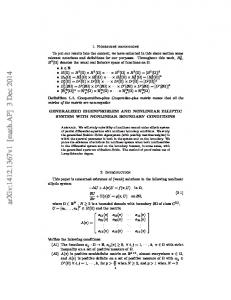
near Γ2,i for some σ > 0 and positive constants C1 , C2 , then (uλ,µ , vλ,µ ) converges + + uniformly on compacts of the remaining components Ω+ i ∪Γi where µ > µi to a weak solution of the system  ∂u   ∆u = a(x)up v q in Ω+ u = ∞ on Γ2,i , = λ1 u on Γ+ i , i , ∂ν (1.8) ∂v   ∆v = b(x)ur v s in Ω+ , v = 0 on Γ2,i , = µv on Γ+ i i , ∂ν where Γ2,i := ∂Ω+ i ∩ Γ2 . B) Assume λ1 = ∞. (iii) If 0 < r < (p − 1)/2, then (uλ,µ , vλ,µ ) converges uniformly in compacts of Ω to the unique positive weak solution (u∞,µ , v∞,µ ) of the system   ∆u = a(x)up v q in Ω u = ∞ on ∂Ω ∂v  ∆v = b(x)ur v s in Ω = µv on ∂Ω, ∂ν as λ → +∞. (iv) If r ≥ (p − 1)/2, then uλ,µ → +∞ and vλ,µ → 0 uniformly in Ω as λ → +∞. Remark 2. In the case Ω+ ⊂⊂ Ω (and so λ1 < ∞) no special values of µ have influence on the limit behavior of the solutions and the conclusion of i) holds true. Statements symmetric to those in (iii) and (iv) hold when λ is kept fixed and µ → +∞. Thus it only remains to study the behavior of (uλ,µ , vλ,µ ) when both λ and µ go to infinity. Accordingly, the existence of positive solutions is required for λ, µ free of upper limitations. Thus, as the weights a and b are not playing now a significative role, we are setting in the remaining statements a(x) = b(x) = 1 (as a minor remark, observe that solutions are now classical thanks to standard elliptic theory, see [1], [21] and [22]). We show that, depending on the relative values of p, q, r, s and on the quotients λ/µ, µ/λ, the solutions converge to a finite profile or not. We remark that uniqueness of positive classical solutions to the system (1.9) below was proved in [16]. Theorem 5. Assume a(x) = b(x) = 1, and let (uλ,µ , vλ,µ ) be the unique positive weak solution to (1.1)-(1.2). (i) If r < (p − 1)/2, q < (s − 1)/2, then (uλ,µ , vλ,µ ) converges uniformly on compacts of Ω to the unique positive weak solution (u∞ , v∞ ) to ½ ∆u = up v q in Ω, u = ∞ on ∂Ω, (1.9) ∆v = ur v s in Ω, v = ∞ on ∂Ω, as λ, µ → ∞.

AN ELLIPTIC SYSTEM

r

7

r

rq = (p-1)(s-1)

rq = (p-1)(s-1)

p-1

p-1

(p-1)/2

(p-1)/2

(s-1)/2

s-1

q

(s-1)/2

s-1

q

Figure 3. On the left we highlight the regions of parameters corresponding to the asymptotic behaviors described in points i) and ii) of Theorem 5 and on the right the parametric regime leading to the behavior in iii).

(ii) If r < p − 1, q < s − 1 and λ, µ → ∞ in such a way that µ/λ is bounded and bounded away from zero, then (uλ,µ , vλ,µ ) converges uniformly on compacts of Ω to the unique positive weak solution (u∞ , v∞ ) to (1.9). (iii) If r > p − 1 (resp. q > s − 1) and λ, µ → ∞ in such a way that µ/λ (resp. λ/µ) is bounded, then uλ,µ → +∞, vλ,µ → 0 (resp. uλ,µ → 0, vλ,µ → +∞) uniformly in Ω. As a complement of the behavior observed in point ii) of the precedent theorem, we show that even in the regime r < p − 1, s < q − 1, solutions do not converge to a finite profile as λ, µ → ∞ provided λ, µ vary along some curves of the form µ = Cλθ for certain values of θ ∈ (0, 1). Such conclusion is attained under radial symmetry on x. However, we suspect that a similar assertion is true in any smooth bounded domain of RN . Theorem 6. Assume (p − 1)/2 < r ≤ p − 1 and choose µ = Cλθ for any constant C > 0 and (1.10)

0 0 on ∂Ω then we also have the complementary upper estimate ³ α ´−2/(p−1) 0 (2.5) Uλ (x) ≤ C d(x) + λ in Ω, for λ ≥ λ0 , where C 0 is a positive constant which does not depend on λ.

AN ELLIPTIC SYSTEM

9

Remark 3. To simplify somewhat the notation, we will denote by Vµ the unique solution to the corresponding problem for v where b(x), s, µ replace a(x), p, λ in (2.1). More precisely,   ∆v = b(x)v s in Ω, (2.6) ∂v  = µv on ∂Ω. ∂ν Proof. Our analysis in [17] dealt with existence, uniqueness and limit profile properties of classical solutions to the more regular version of (2.1) where a ∈ C α (Ω) for some 0 < α < 1. In addition, the existence of a H 1 weak solution to (2.1) was obtained there by a variational approach covering the more general framework a ∈ L∞ (Ω). Furthermore, it was shown in [19] (see also [20]) that H 1 solutions are also in L∞ (Ω) and so they are unique and define strong solutions (see above) to (2.1). Therefore, we are only proving (2.2), (2.4) and (2.5), the remaining assertions being essentially contained in Theorems 1, 2 and 3 of [17]. To show (2.2), let λn → 0, and denote for simplicity un = Uλn . Proceeding as in the proof of Theorem 1 in [17] it follows that |un |∞ → 0. Thus vn := un /|un |∞ solves ( p ∆v = a(x)|un |p−1 in Ω, ∞ v ∂v (2.7) = λn v on ∂Ω. ∂ν The right-hand side of the equation in (2.7) is bounded and so, also proceeding as in [17], one obtains a subsequence, still named vn , such that vn → v in C 1,η (Ω) for every η ∈ (0, 1), being v a strong solution to ( ∆v = 0 in Ω, ∂v = 0 on ∂Ω, ∂ν with |v|∞ = 1. Hence v = 1. On the other hand, integrating the equation in (2.7) we get Z Z p−1 λn vn = |un |∞ a(x)vnp−1 , ∂Ω

and we arrive at

Ω

1 ¶− p−1 Z 1 1 un ∼ |un |∞ ∼ a(x) λnp−1 . ∂Ω Ω Since the sequence λn is arbitrary, this proves (2.2). To prove (2.4), we construct a suitable subsolution in a neighborhood of the boundary. Since Ω is C 2 , there exists δ0 such that d(x) is C 2 in 0 < d < δ0 and |∇d| = 1 there (cf. [21]). We search for our subsolution in the form

(2.8)

µ

u = ε(d(x) + θ)−α ,

where ε is small, α = 2/(p − 1) and θ > 0 is to be chosen. On the boundary we have, ¶ µ ¶ µ ¯ ¯ ¢ ¡ ∂u ∂u ¯ − λu ∂Ω = − − λu ¯d=0 = ε αθ−α−1 − λθ−α , ∂ν ∂d so it suffices with setting θ = α/λ. On the other hand: ∆u − a(x)up = ε(d + θ)−α−2 (α(α + 1) − α(d + θ)∆d − a(x)εp−1 ). Thus u will be a subsolution provided ³ ´ α α (α + 1) − (d + )∆d ≥ εp−1 sup a. λ 0 0 in ∂Ω, a supersolution similar to the subsolution in (2.8) can be constructed near ∂Ω, so the proof of (2.5) is entirely similar. We leave the details to the reader. ¤ We are now concerned with a more general version of problem (2.1). We are allowing the weight a(x) to be discontinuous but keeping its boundedness. We also assume that it depends on a parameter ε and becomes singular –in two different possible ways– as ε → 0. More precisely, we consider   ∆u = Aε (x)us in Ω, (2.9)  ∂u = µu on ∂Ω, ∂ν s > 1, µ > 0, where we are assuming that Aε ∈ L∞ (Ω), ε > 0, is a family of bounded functions which verify either of the two following conditions. Namely, (2.10)

Aε (x) → ∞ uniformly in Ω0

as ε → 0 in a smooth subdomain Ω0 of Ω satisfying the structure conditions of Ω0 in 0 hypothesis (H) (cf. Section 1). In this scenario we define Ω00 = Ω \ Ω and we are supposing in addition that Aε remains uniformly bounded in Ω00 . An alternative condition that we are studying is (2.11)

Aε (x) ≥ C (d(x) + ε)−θ

in Ω

for a certain θ ≥ 1 and a positive constant C. We are interested in analyzing the behavior of the unique positive solution Uµ,ε to (2.9) as ε → 0, for fixed µ > 0. We remark that the results in Theorem 7 still hold for bounded weights with no essential modifications. The main features of problem (2.9) when the coefficient Aε behaves in the singular way that are described below.

AN ELLIPTIC SYSTEM

11

Theorem 8. Suppose Aε ∈ L∞ (Ω), ε > 0, is a family of functions such that Aε (x) decreases 0 in ε > 0, verifies (2.10) and remains uniformly bounded in Ω \ Ω . Then the unique solution 0 u = Uµ,ε to (2.9) converges uniformly to zero in Ω as ε → 0. Furthermore, Uµ,ε also converges uniformly to zero in every connected piece Ω00i of Ω00 such that µ ≤ µ1,i where µ1,i = ∞ if Ω00i ⊂⊂ Ω or µ = µ1,i stands for the principal eigenvalue to the problem ([17], [18])   ∆ψ = 0 x ∈ Ω00i ,    ψ=0 x ∈ ∂Ω00i ∩ Ω,     ∂ψ = µψ x ∈ ∂Ω00i ∩ ∂Ω. ∂ν Proof. We are using the notation uε instead Uµ,ε for simplicity. In addition we put Γ01 = ∂Ω0 ∩ Ω, Γ00 = ∂Ω00 ∩ ∂Ω, Γ0 = ∂Ω0 ∩ Ω = ∂Ω00 ∩ Ω. Remark that, according to (H), Γ0 ⊂ Ω is a closed manifold which is always nonempty while either Γ01 or Γ00 could be possibly empty, but not simultaneously. We are next dealing with the more elaborate case where both Γ01 and Γ00 are nonempty (the remaining possibilities are handled in the same way). We also denote A0 (x) = supε>0 Aε (x) = limε→0 Aε (x) for x ∈ Ω00 . Observe that A0 ∈ L∞ (Ω00 ). The auxiliary problem:   ∆u = A0 us x ∈ Ω00 ,    u=0 x ∈ Γ0 , (2.12)     ∂u = µu x ∈ ∂Ω00 , ∂ν 00

has a unique positive strong solution uˆ0 ∈ W 2,p (Ω00 ) ∩ C 1,η0 (Ω ) for every p > 1, 0 < η0 < 1. On the other hand, the positive strong solution uε to (2.9) belongs to W 2,p (Ω) ∩ C 1,η0 (Ω), p > 1, 0 < η0 < 1, and is increasing in ε. Therefore the function u0 given as u0 (x) = lim uε (x) = inf uε (x),

x ∈ Ω,

ε>0

is well defined, lies in L∞ (Ω) while the limit holds in Lp (Ω) for all p ≥ 1. We are next showing that u0 = 0 a. e. in Ω0 together with u0 (x) = uˆ0 (x) for all x ∈ Ω00 . First, observe that uˆ0 ∈ HΓ10 (Ω00 ) = {u ∈ H 1 (Ω00 ) : u|Γ0 = 0} defines the minimum of the variational problem inf J0 (u), 1 u∈HΓ0 (Ω00 )

where, 1 J0 (u) = 2

Z

1 |∇u| + s+1 Ω00

Z

2

A0 u Ω00

s+1

µ − 2

Z u2 . Γ00

Similarly, Jε (uε ) = inf H 1 (Ω) Jε (u) where Z Z Z 1 1 µ 2 s+1 Jε (u) = |∇u| + Aε u − u2 . 2 Ω s+1 Ω 2 ∂Ω Thus, by letting u0 ∈ H 1 (Ω) be the extension by zero of uˆ0 to Ω, we achieve (2.13)

Jε (uε ) ≤ Jε (u0 ) ≤ J0 (ˆ u0 )

ε > 0.

12

´ J. GARC´IA-MELIAN, J. D. ROSSI AND J. C. SABINA DE LIS

This implies the boundedness of uε in H 1 (Ω), hence uε * u0 and so u0 ∈ H 1 (Ω). It follows in addition from (2.13) that Z mε us+1 = O(1) as ε → 0, ε Ω0

with mε → ∞. From this u0 = 0 a. e. in Ω0 which implies that the restriction of u0 to Ω00 belongs to HΓ10 (Ω00 ). By taking now limits in (2.13) we obtain J0 (u0 ) ≤ J(ˆ u0 ). From the uniqueness of the weak solution to (2.12) we conclude u0 = uˆ0 a.e. in Ω00 . However, the interior version of the W 2,p estimates in [1] can be used to show that the convergence uε → u0 actually occurs in C 1,η0 (Ω00 ∪ Γ00 ), 0 < η0 < 1. Thus u0 ∈ C 1,η0 (Ω00 ∪ Γ00 ) which in turn ensures that u0 (x) = uˆ0 (x) for every x ∈ Ω00 . 0 Let us finish by showing the uniform convergence of uε to zero in Ω . For δ > 0 small define Qδ = {x ∈ Ω : dist (x, Ω0 ) < δ} the δ neighborhood of Ω0 in Ω, Γ0δ = {x ∈ ∂Qδ : dist (x, Ω0 ) = δ}. Observe that −∆uε + muε ≤ muε , for m > 0 conveniently large, so that we achieve uε (x) ≤ u˜ε,δ (x)

x ∈ Qδ ,

where u = u˜ε,δ ∈ C 1,η0 (Qδ ) stands for the strong positive solution to the problem   −∆u + mu = muε x ∈ Qδ ,    u = uε x ∈ Γ0δ , (2.14)   ∂u   = µu x ∈ Γ01 . ∂ν Observe now that Γ0δ ⊂ Ω00 and thus we get uniform estimates of the W 2−1/p,p (Γ0δ ) norm of uε . By employing the W 2,p estimates in [1] we conclude that u˜ε,δ → u˜0,δ in C 1,η0 (Qδ ), being u˜0,δ the strong solution to the problem   x ∈ Qδ , −∆u + mu = mu0    u = uˆ0 x ∈ Γ0δ , (2.15)     ∂u = µu x ∈ Γ01 . ∂ν Therefore, (2.16)

u0 (x) ≤ u˜0,δ (x)

for all x ∈ Qδ . 0

We are finally proving that u˜0,δ converges uniformly to zero in Ω as δ → 0. In fact, a smooth 0 0 family of diffeomorphisms x = Tδ (y), Tδ : Ω → Qδ exists which leave invariant Ω \ Uδ , Uδ a small δ-varying neighborhood of Γ0δ in Qδ and such that Tδ (Γ0 ) = Γ0δ for every δ > 0 (see [25]). Setting y = Hδ (x) := Tδ−1 (x) the inverse diffeomorphism, the “mayorant” problem

AN ELLIPTIC SYSTEM

(2.15) is transformed into (2.17)  N N X X  ∂ 2v ∂v    − ∆(Hδ )k + mv = mu0 (Tδ (y)) − h∇(H ) , ∇(H ) i δ k δ l   ∂yk ∂yl k=1 ∂yk  k,l=1

13

y ∈ Ω0 ,

v = uˆ0 (Tδ (y)) y ∈ Γ0 ,        ∂v = µv x ∈ Γ01 . ∂ν The unique strong solution to (2.17) is provided by vδ = u˜0,δ ◦ Tδ . Since uˆ0 ∈ W 2,p (Ω00 ) ∩ 00 C 1,η0 (Ω ) we are in possession of uniform bounds in W 2−1/p,p (Γ0 ) of uˆ0 ◦ Tδ . Therefore, the 0 W 2,p estimates in [1] once again imply the convergence vδ → v0 in W 2,p (Ω0 ) ∩ C 1,η0 (Ω ) where v0 is the unique solution of the limit problem obtained from (2.17) as δ → 0. Taking into account that h∇(Hδ )k , ∇(Hδ )l i = δkl and ∆(Hδ )k = 0 at δ = 0 or 1 ≤ k, l ≤ N ([25]) the limit problem becomes   −∆v + mv = 0 x ∈ Ω0    v=0 x ∈ Γ0 (2.18)     ∂v = µv x ∈ Γ01 . ∂ν However, if m is large enough the unique solution of (2.18) is v0 = 0. Therefore and taking limits in (2.16) as δ → 0 it is obtained that u0 = 0 at every x ∈ Ω0 . The uniform character of the convergence uε → 0 in Ω0 is implicit in the preceding argument. Alternatively, Dini’s theorem can be employed. At the present moment Ω00 has been regarded as a “whole”. The proof of the theorem is completed with the additional remark that uˆ0 = 0 at every connected piece Ω00i of Ω00 such that either Ω00i ⊂⊂ Ω0 or µ ≤ µ1,i (cf. [17]). ¤ A second result describing the behavior of positive solutions to problem (2.9) when the weight Aε develops a singularity on the boundary is the following. Theorem 9. Consider a family Aε ∈ L∞ (Ω), ε > 0, which is decreasing in ε and verifies the condition (2.11) for a certain θ ≥ 1 while u = Uµ,ε stands for the unique positive solution to (2.9). Then Uµ,ε → 0 uniformly in Ω as ε → 0. Proof. To simplify, let us define as before uε = Uµ,ε the unique positive solution to (2.9). Since Aε is decreasing in ε, uε is increasing in ε, and then uε → u0 as ε → 0, where u0 is a nonnegative function. In addition, such a convergence holds in Lp (Ω) for all p > 1 while proceeding as in the proof of Theorem 8 it follows that both uε → u0 weakly in H 1 (Ω) and in C 1,η0 (Ω), 0 < η0 < 1. We deduce from (2.9) and (2.11) that Z Z Z Z Z 2 −θ s+1 2 2 s+1 u2ε . uε − |∇uε | ≤ µ C (d(x) + ε) uε ≤ Aε (x)uε = µ s + 1 Ω ∂Ω ∂Ω Ω Ω We can now pass to the limit as ε → 0, use Fatou’s theorem and obtain Z Z −θ p+1 (2.19) C d(x) u0 ≤ µ u20 . Ω

∂Ω

We claim that the convergence of the integral in the right-hand side of (2.19) implies, in view of θ ≥ 1, that u0 = 0 on ∂Ω. Thus (2.19) and the continuity of u0 readily give u0 (x) = 0

14

´ J. GARC´IA-MELIAN, J. D. ROSSI AND J. C. SABINA DE LIS

for every x ∈ Ω. We are next showing the uniform convergence to zero in Ω. First, u = uε satisfies for 0 < ε < ε0 , −∆u + mu ≤ mu, for a conveniently large m. That is why uε (x) ≤ uˆε (x)

for all x ∈ Ω,

where u = uˆε is the unique strong (even classical!) solution to the majorant problem  x ∈ Ω0 , −∆u + mu = muε (2.20)  ∂u = µu x ∈ ∂Ω. ∂ν By arguing as in the proof of Theorem 8 it follows that uˆε converges in C 1,η0 (Ω) to the unique solution uˆ0 to the limit problem of (2.20), namely  x ∈ Ω0 , −∆u + mu = 0  ∂u = µu x ∈ ∂Ω. ∂ν Choosing a large m guarantees that uˆ0 (x) = 0 for every x ∈ Ω and so uε → 0 uniformly in Ω. We finally outline the proof of the claim: observe first that if Ra nonnegative u lies in say ρ 1 H (I), I = (0, 1) the unit interval, and makes finite the integral 0 x−θ u(x) dx for a certain ρ > 0 then, since u ∈ C[0, 1], u(0) must be necessarily zero provided θ ≥ 1. In the N dimensional case above, after a change of variables near the boundary, u0 belongs to H 1 (Iδ ) where Iδ stands for a uniform one-dimensional interval of length δ > 0 on the normal inner semiline to ∂Ω, for “almost all normal lines”, the “almost all” being considered with respect to the N − 1 dimensional measure on ∂Ω. Moreover, an integral exactly as the considered above must be finite for almost all those normals. Therefore, u0 (x) = 0 for almost all x ∈ ∂Ω and we are done. ¤ Our next step is to consider problem (2.1), when the weight is allowed to be singular on ∂Ω, that is, we study ( ∆v = B(x)v s in Ω, ∂v (2.21) = µv on ∂Ω, ∂ν where the weight B(x) is a continuous, positive function in Ω, and we require an upper bound for the singularity of the form (2.22)

B(x) ≤ Cd(x)−τ

for some τ < 1 and C > 0 (for its use in Section 4, we have replaced a(x), p, λ by B(x), s, µ). Then we have the following result. Theorem 10. Let B be a positive continuous function in Ω which verifies (2.22). Then problem (2.21) admits a unique positive weak solution V˜µ ∈ H 1 (Ω) ∩ L∞ (Ω) for every µ > 0. Moreover, V˜µ is increasing in µ and converges as µ → ∞ to the minimal positive solution V˜∞ to ½ ∆V = B(x)V s in Ω, (2.23) V =∞ on ∂Ω.

AN ELLIPTIC SYSTEM

15

Proof. Let us first show existence. We truncate the weight B multiplying by a smooth cut-off function. To this aim, let ψ ∈ C ∞ (R) such that 0 ≤ ψ ≤ 1, ψ(t) = 0 if t ≤ 1 while ψ(t) = 1 for t ≥ 2, and ψ is increasing. If we denote Bk (x) = ψ(kd(x))B(x), we obtain a family of increasing, bounded weights such that Bk → B uniformly on compacts of Ω as k → ∞. We consider the truncated problem ( ∆v = Bk (x)v s in Ω, ∂v (2.24) = µv on ∂Ω, ∂ν which has a unique positive weak solution vk for every µ > 0, thanks to Theorem 7. Moreover, vk is decreasing in k, since vk+1 is a subsolution to problem (2.24) while M vk is a supersolution with a large enough M . To be able to pass to the limit, we need a uniform subsolution, to guarantee that vk is bounded away from zero. Recall that Bk (x) ≤ B(x) ≤ Cd(x)−τ , and let φ be the unique (positive) solution to the equation ½ −∆φ = Cd(x)−τ in Ω, (2.25) φ=0 on ∂Ω. We remark that (2.25) has a solution φ ∈ C 1,1−τ (Ω) since τ < 1, thanks to Theorem 8.34 in [21]. We are taking the subsolution as v = ε − εs φ, for small positive ε. We have ∆v = εs Cd(x)−τ ≥ εs Bk (x) ≥ Bk (x)εs (1 − εs−1 φ)s = Bk (x)v s , in Ω, while ∂v ∂φ = −εs ≤ µε = µv ∂ν ∂ν on ∂Ω, for small ε. Since there are large supersolutions, we deduce vk ≥ v in Ω. Moreover: Z Z Z Z s+1 2 2 |∇vk | = µ vk − Bk (x)vk ≤ µ vk2 , Ω

∂Ω

Ω

1

∂Ω

2

so that vk → v weakly in H (Ω), strongly in L (Ω), and v ≥ v. In particular, since for every ψ ∈ H 1 (Ω) we have Z Z Z (2.26) ∇vk ∇ψ − µ vk ψ = Bk (x)vks ψ Ω

∂Ω

Ω

and 0 ≤ Bk ≤ B ∈ L1 (Ω) (due to τ < 1), the dominated convergence theorem allows us to pass to the limit in (2.26) and obtain that v is a weak positive solution to (2.21). To show uniqueness we first observe that every nonnegative weak solution w ∈ H 1 (Ω) to (2.21) lies necessarily in L∞ (Ω) (see [20]). This in particular implies, in virtue of the uniqueness of solutions to (2.24) that w ≤ v. If, however, w is nontrivial (and so positive) since B ∈ L1 (Ω), we can argue as in [17] to obtain that w = v. Thus problem (2.21) admits a unique positive solution. Finally, the asymptotic behavior of V˜µ is obtained as in [17] (we refer also to [4] for ¤ existence and uniqueness results on problem (2.23) and related ones). Another problem that will be necessary in Section 4 is obtained when the weight function is supported in a subdomain Ω+ of Ω, and different boundary conditions are imposed on two parts of ∂Ω+ . More precisely, we are interested in the case Ω+ = Ω \ Ω0 , where Ω0 is the same as in hypothesis (H) on a(x) and Ω+ might exhibit multiple connected pieces Ω+ i .

16

´ J. GARC´IA-MELIAN, J. D. ROSSI AND J. C. SABINA DE LIS

Recalling the notation Γ+ = ∂Ω+ \ Γ2 (with Γ2 = ∂Ω0 ∩ Ω) we are dealing with the following problem, related to (2.1) but with a singular boundary condition  ∆w = A(x)wp in Ω+ ,    w=∞ on Γ2 , (2.27)  ∂w   = λw on Γ+ . ∂ν The function A(x) essentially behaves as a power of the distance d(x) = dist(x, Γ2 ). Problem (2.27) for bounded weights was considered in [17] (although no estimates were provided there). We are also including here for completeness the case of singular weights. Our result for problem (2.27) is as follows. Theorem 11. Let A be a continuous positive function in Ω+ ∪ Γ+ such that C1 d(x)τ ≤ A(x) ≤ C2 d(x)τ , d(x) = dist(x, Γ2 ), for some positive constants C1 , C2 and τ > −2. Then the problem (2.27) admits a unique positive weak solution wλ . Moreover, there exist positive constants D1 , D2 such that (2.28)

2+τ

2+τ

D1 d(x)− p−1 ≤ wλ (x) ≤ D2 d(x)− p−1

x ∈ Ω.

Proof. The proof is an adaptation of that of Theorem 1 in [4]. We may assume τ < 0, since when τ ≥ 0 the existence result is contained in [17]. We first fix n ∈ N and truncate the weight A(x) as in the proof of Theorem 10 to obtain a bounded weight Ak (x) and deal with the family of problems,  ∆w = Ak (x)wp in Ω+ ,    w=n on Γ2 , (2.29)  ∂w   = λw on Γ+ . ∂ν Problem (2.29) admits for every k, n ∈ N a unique strong solution wk,n , which is in addition unique thanks to Lemma 8 in [17]. In fact, w = 0 is a subsolution. To construct large supersolutions we distinguish two cases. For λ > λ1 , λ1 the principal eigenvalue to (1.5) regarded in Ω+ , and a small enough δ, the problem  ∆u = Ak (x)up in Ω+  δ ,   u=0 on Γ2,δ ,  ∂u   = λu on Γ+ , ∂ν + with Ω+ δ = Ω ∪ Γ2 ∪ {x : dist (x, Γ2 ) < δ}, Γ2,δ = {x ∈ ∂Ωδ : dist (x, Γ2 ) = δ} admits a unique positive strong solution uλ,δ . To see this it suffices with proceeding as in [17] where an entirely similar problem is considered. Thus, since uλ,δ is positive on Γ2 , w = M uλ,δ defines, for large M > 0, a supersolution as large as desired. In the second case, where λ ≤ λ1 and a small enough δ > 0 again, the eigenvalue problem ([17])  ∆φ = σφ in Ω+  δ ,   φ=0 on Γ2,δ ,  ∂φ   = λφ on Γ+ , ∂ν

AN ELLIPTIC SYSTEM

17

admits a unique principal eigenvalue σ = σ1 < 0 with a positive associated eigenfunction φ1,δ . Being φ1,δ positive on Γ2 it then clear that w = M φ1,δ defines a large supersolution to (2.29) modulated by M > 0. Notice in addition that this choice of w also works in the present case for λ > λ1 since A is positive in Ω (our previous construction covers A nonnegative). Moreover, since Ak is increasing in k, wk,n is decreasing in k, and it is increasing in n. By fixing n it follows that wk,n converges in C 1,η0 (Ω+ ∪ Γ+ ) ∪ W 2,q (Ω+ ∩ {d > δ}) to a strong solution wn of the equation satisfying the flux condition. To achieve the continuity up to Γ2 we can now argue as in [4] to construct a local barrier near Γ2 . Thus we obtain that wn defines a strong solution to  ∆w = A(x)wp in Ω+ ,    w=n on Γ2 ,  ∂w   = λw on Γ+ . ∂ν In addition, wn is increasing in n. Since A(x) ≥ A0 > 0 in Ω, it follows that wn is locally bounded in Ω. Indeed, the upper bound is provided by the minimal solution to the previous problem with A(x), n replaced by A0 , ∞, respectively. Thus we can pass to the limit to obtain that wn → w locally uniformly, where w is a weak solution to (2.27). Estimates (2.28) are proved exactly as in Theorem 3.1 in [4] (we remark that the estimates are local in nature). Finally, the uniqueness is a consequence of the estimates (2.28) by proceeding as in Theorem 3.4 of [4]. ¤ We finally turn to consider the perhaps most interesting of our auxiliary problems. In this case, the weight is singular on Γ2 (behaving essentially as a power of the distance d(x) = dist(x, Γ2 )) and a homogeneous Dirichlet condition is imposed there. Such boundary condition makes that the problem can always be solved independently of the singularity of the weight, in contrast for example with Theorem 11. Imitating our framework described in hypothesis (H) we are considering a bounded smooth domain Ω+ (in future applications such domain will be a connected piece of {a > 0}) whose boundary splits off in two separate groups Γ2 , Γ+ , of closed N − 1 dimensional manifolds. Our next problem will be,  ∆z = B(x)z s in Ω+ ,    z=0 on Γ2 , (2.30)    ∂z = µz on Γ+ , ∂ν with B positive and continuous in Ω+ ∪ Γ+ but singular on Γ2 . As mentioned above, the case where B is continuous up to Γ2 can be treated as in [17], to show that there exists a unique weak solution provided µ > µ+ , where µ = µ+ is the principal eigenvalue of the problem  ∆φ = 0 in Ω+ ,    φ=0 on Γ2 ,    ∂φ = µφ on Γ+ . ∂ν When B is singular, the existence of solutions is not at all straightforward. We remark that the hard task in this case is to obtain estimate near Γ2 for the (unique) solution. These estimates will be important later on.

18

´ J. GARC´IA-MELIAN, J. D. ROSSI AND J. C. SABINA DE LIS

Theorem 12. Let B be continuous and positive in Ω+ ∪ Γ+ , and assume there exist positive constants C1 , C2 and τ such that C1 d(x)−τ ≤ B(x) ≤ C2 d(x)−τ

x ∈ Ω+ ,

where d(x) = dist(x, Γ2 ). Then problem (2.30) can only have positive solutions if µ > µ+ and in fact such solutions exist for each µ > µ+ . Furthermore, provided τ 6= s + 1, positive weak solutions are unique in that range. More importantly, if z = zµ stands for the solution to (2.30), then there exist positive constants D1 , D2 such that D1 d(x)θ ≤ zµ (x) ≤ D2 d(x)θ

(2.31)

in Ω, where θ = max{1, (τ − 2)/(s − 1)}. Remark 4. A close analysis of symmetric cases shows that estimates (2.31) fail when τ = s+1 and in fact zµ decays near Γ2 as h(d)d with h involving a negative power of log d−1 . However, since this precise information is not to be used in this paper we are not sharpening the estimates in this case. Proof of Theorem 12. Let us show that no positive solutions exist when µ ≤ µ+ . Assume + there exists a positive weak solution z to (2.30). Let Ω+ : d(x) > 1/n}, n = {x ∈ Ω + d(x) = dist(x, Γ2 ), and µn , φn the principal eigenvalue and corresponding eigenfunction in Ωn of  in Ω+  n,  ∆φ = 0  φ=0 on Γ2,n ,    ∂φ = µφ on Γ+ , ∂ν + + where Γ2,n = ∂Ω+ \ Γ . It is not hard to show that µ+ n n → µ , while φn → φ uniformly on compacts of Ω+ ∪ Γ+ (notice that only the Dirichlet boundary condition is perturbed). If we multiply (2.30) by φn and integrate in Ω+ n we get, Z Z Z ∂φn s + B(x)z φn = (µ − µn ) (2.32) zφn − z. Ω+ Γ+ Γ2,n ∂ν n The last term goes to zero as n → ∞. Indeed, notice that estimates (2.31) – which will be + proved later on – imply that z ∈ C(Ω ) and z = 0 on Γ2 in the usual pointwise sense. Thus, given a small ε > 0 and taking a large enough n we can assume that 0 < z ≤ ε on Γ2,n . Thus, ¯Z ¯ Z Z Z ¯ ∂φn ¯¯ ∂φn ∂φn ¯ + z ¯ ≤ −ε =ε = εµn φn = O(ε), ¯ ¯ Γ2,n ∂ν ¯ Γ2,n ∂ν Γ+ ∂ν Γ+ as ε → 0+. Since ε is arbitrary, we can pass to the limit in (2.32) by means of the dominated convergence theorem to arrive at Z Z s + B(x)z φ = (µ − µ ) zφ, Ω+ +

Γ+

and we deduce µ > µ , since z and φ are strictly positive on Γ+ . Now assume µ > µ+ , and let us show that there exists a positive solution to (2.30). Since + B(x) is bounded in Ω+ n and µ > µn for a sufficiently large n, it follows that (2.30) has a + + solution in Ω+ n (by replacing Ω by Ωn and Γ2 by Γ2,n ). This solution is in addition unique, thanks to Lemma 8 in [17]. Let us denote it by zn . We have zn ≤ zn+1 , since zn+1 is a supersolution to the problem in Ω+ n , while εzn is a subsolution for small positive ε. On the

AN ELLIPTIC SYSTEM

19

other hand, it is possible to obtain a uniform bound by taking M Zµ , where Zµ is the solution to (2.30) with B ≡ 1 (notice that Zµ > 0 on Γ2,n ) where M is large and independent of n. We deduce then that zn ≤ M Zµ . It is now standard to conclude that zn → z in C 1 (Ω+ ∪Γ+ ), where z is a positive weak solution to (2.30). Notice that z = 0 on Γ2 , since z ≤ M Zµ and Zµ = 0 on Γ2 . Let us now prove that every positive solution to (2.30) satisfies the estimates (2.31). Notice first that, thanks to Hopf’s maximum principle, Zµ (x) ≤ Cd(x). Thus, every positive solution z verifies z ≤ Cd. Now we use an argument from [4]. Take x near Γ2 , and introduce the function w(y) = d(x)−σ z(x + d(x)y) with σ = (τ − 2)/(s − 1) and y ∈ B1/2 (0). We have ∆w ≥ Cws in B1/2 (0), and hence w ≤ W , the unique solution to ∆W = CW s in B1/2 with W|∂B1/2 = ∞. Setting y = 0, we arrive at z(x) = w(0)d(x)σ ≤ W (0)d(x)σ . Thus we have shown z(x) ≤ Cd(x)θ , where θ = max{1, (τ − 2)/(s − 1)}. The lower estimate is more delicate. If σ > 1, it is easily seen that u = εd(x)σ is a subsolution in a neighborhood of Γ2 of the form 0 < d < δ provided ε and δ are small enough. Indeed, ∆u − B(x)us ≥ εσ(σ − 1)dσ−2 + εσdσ−1 ∆d − Cεs d−τ +sσ = εdσ−2 (σ(σ − 1) + σd∆d − Cεs−1 ), and this quantity can be made positive when σ > 1, by taking ε and δ adequately small. Now let z be a positive solution to (2.30). Then w = z clearly satisfies (d = dist(x, Γ2 ))  s   ∆w = B(x)w in 0 < d < δ, w=0 on d = 0,   w=z on d = δ. By diminishing ε if necessary, we can achieve u < z on d = δ. This implies u ≤ z in 0 < d < δ. In fact, let D = {u > z} ∩ {0 < d < δ}, and assume D 6= ∅. In D we have ∆u > ∆z, and by the maximum principle, since u = z on ∂D, we arrive at u ≤ z in D, which is impossible. Hence, D = ∅, that is, z ≥ u, so that z(x) ≥ Cd(x)σ , provided σ > 1. We are now considering the case σ < 1. For x0 ∈ Γ2 , take an annulus A = {x : R1 < |x − x˜| < R2 }, tangent to Γ2 at x0 , and such that A ⊂ Ω+ . With no loss of generality, we can assume x˜ = 0. Consider the problem  −τ s   ∆w = C(R2 − |x|) w in A, w=ε on |x| = R1 , (2.33)   w=0 on |x| = R2 , where C > 0 and ε is sufficiently small. Problem (2.33) has at least a radial solution w, which can be constructed as before, by approximating A by sub-annulus which avoid the boundary |x| = R2 . Moreover, it follows again that z ≥ w. Notice in addition that w ≤ C(R2 − r).

20

´ J. GARC´IA-MELIAN, J. D. ROSSI AND J. C. SABINA DE LIS

Let us obtain a lower estimate for w near |x| = R2 . To this aim, we perform in the radial version of (2.33) the change of variables:  µ ¶ 1 1 1   − N −2 N ≥ 3,  N −2 N− R2 µ 2 ¶r y= R2   N = 2,  log r where r = |x|, and obtain, in the new variable y: ½ 00 w = b(y)ws , w(0) = 0,

y > 0,

where b(y) is continuous in y > 0 and verifies C1 y −τ ≤ b(y) ≤ C2 y −τ near y = 0. Also, w(y) ≤ Cy, and we have to prove that w(y) > 0. y→0 y Notice first of all that w is convex. Thus, w0 is increasing and we deduce that necessarily w0 ≥ 0 for y > 0 small, since w(0) = 0 and w > 0. Moreover, w0 has a limit at y = 0. Assume for a contradiction that (2.34) does not hold, so that limy→0 w0 (y) = 0. Choose y0 > 0 and integrate the equation between y0 and y; we obtain: Z yZ t 0 w(y) = w(y0 ) + w (y0 )(y − y0 ) + b(r)w(r)s drdt. (2.34)

lim inf

y0

y0

Let wδ = sup[0,δ] w(y)/y. We already know that wδ ≤ C for sufficiently small δ. Hence: w(y) ≤ w(y0 ) + w0 (y0 )(y − y0 ) + Cwδs ((y −τ +s+2 − y0−τ +s+2 ) − y0−τ +s+1 (y − y0 )), where C is a positive constant, whose exact value is irrelevant. Now observe that −τ +s+1 > 0 – since σ < 1 – so that, letting y0 → 0 and dividing by y we obtain, w(y) ≤ Cwδs y −τ +s+1 . y Taking supremums and dividing by wδ , we arrive at 1 ≤ Cwδs−1 δ −τ +s+1 , which is a clear contradiction when δ → 0. Thus (2.34) holds. Going back to the original variables, we have shown w(r) ≥ C(R2 − r), so that z(x) ≥ Cd(x). when σ < 1, which concludes the proof of (2.31). Finally we prove uniqueness. Let z, w be positive solutions to (2.30). Thanks to (2.31), it follows that z/w, w/z are bounded functions. Moreover, B(x)z s+1 and B(x)ws+1 are ¤ integrable. Hence, we can proceed as in [17] (see also [3]) to obtain uniqueness. 3. Existence and uniqueness This section is devoted to the proof of Theorem 1. We begin by showing that positive weak solutions exist only when 0 < λ < λ1 ≤ ∞ (see Section 1 for the definition of λ1 ) and µ > 0. Let us remark that, since p, s > 1, the strong maximum principle implies that nonnegative solutions (u, v) to (1.1)–(1.2) verify u > 0, v > 0 in Ω unless u ≡ 0 or v ≡ 0 in Ω. We also mention in passing that when λ = 0 (respectively µ = 0) there exist semitrivial solutions (u, v) = (k, 0), k ∈ R (resp. (u, v) = (0, k 0 ), k 0 ∈ R).

AN ELLIPTIC SYSTEM

21

Lemma 13. Problem (1.1)–(1.2) can only have positive solutions when 0 < λ < λ1 ≤ ∞, µ > 0. Proof. Assume there exists a positive solution (u, v) to (1.1)–(1.2). Integrating the first equation in (1.1) in Ω we get, Z Z p q a(x)u v = λ u, Ω

∂Ω

so that if λ ≤ 0 then u ≡ 0 or v ≡ 0 by the strong maximum principle. This contradicts the positiveness of both u and v. When µ ≤ 0 we proceed similarly. Hence both λ, µ must be positive. Let us see now that 0 < λ < λ1 is also necessary. Denote by φ the positive normalized eigenfunction associated to λ1 . Multiplying the first equation in (1.1) by φ, and then integrating by parts in Ω0 we obtain, Z Z Z ∂φ 0= φ∆u = (λ − λ1 ) uφ − u . Ω0 Γ1 Γ2 ∂ν Since u > 0 in Ω, φ > 0 on Γ1 and ∂φ/∂ν < 0 on Γ2 , we obtain λ < λ1 .

¤

Now we show that when 0 < λ < λ1 , µ > 0, problem (1.1)–(1.2) has at least a positive solution (u, v). We use the notations introduced in Section 2. Lemma 14. Assume 0 < λ < λ1 ≤ ∞, µ > 0. Then problem (1.1)–(1.2) admits a positive weak solution (u, v). Proof. We are obtaining sub and supersolutions by means of the solutions Uλ , Vµ of the auxiliary problems (2.1) and (2.6), respectively. By choosing a small ε and a large M , the pair (εUλ , M Vµ ) defines a subsolution. Notice indeed that the boundary conditions are automatic, while ½ ∆(εUλ ) = εa(x)Uλp ≥ a(x)εp Uλp M q Vµq ∆(M Vµ ) = M b(x)Vµs ≤ b(x)εr Uλr M s Vµs holds provided (3.1)

εp−1 M q sup Vµq ≤ 1, Ω

εr M s−1 inf Uλr ≥ 1. Ω

By setting M = ε−γ , (3.1) can be achieved for small ε if γ is chosen to satisfy p − 1 − γq > 0 > r − γ(s − 1), that is, r p−1 (3.2) 0. A large supersolution is constructed similarly. Hence, for 0 < λ < λ1 , µ > 0, problem (1.1)–(1.2) has a positive solution. ¤ We now turn to consider the question of uniqueness of positive solutions. Although an argument similar to the one employed later on in Section 4 could be used, we prefer to obtain it by means of a sweeping argument. Lemma 15. Assume 0 < λ < λ1 ≤ ∞ and µ > 0 then problem (1.1)–(1.2) admits a unique positive solution (uλ,µ , vλ,µ ). Moreover, (uλ,µ , vλ,µ ) is an asymptotically stable equilibrium for the parabolic system associated to (1.1)-(1.2) which is globally attractive among nonnegative solutions.

22

´ J. GARC´IA-MELIAN, J. D. ROSSI AND J. C. SABINA DE LIS

Proof. Let (u1 , v1 ), (u2 , v2 ) be positive solutions to (1.1)–(1.2). If t ≥ 1 and exponent γ > 0 is selected as in (3.2), (tu1 , t−γ v1 ) is a supersolution. Indeed: ½ ∆(tu1 ) = ta(x)up1 v1q ≤ a(x)tp up1 t−γq v1q ∆(t−γ v1 ) = t−γ b(x)ur1 v1s ≥ b(x)tr ur1 t−γs v1s holds provided tp−1−γq ≥ 1, tr−γ(s−1) ≤ 1, that is, when t ≥ 1, while the boundary conditions remain unchanged. We now use a sweeping argument. If t is large enough, we have tu1 > u2 , t−γ v1 < v2 . Set t0 = inf{t > 1 : tu1 > u2 , t−γ v1 < v2 }. We claim that t0 = 1. To prove the claim, choose M > 0 such that the function f (τ ) = a(x)τ p v2q − M τ is decreasing (with fixed x) in the interval [inf u2 , sup(t0 u1 )]. Then q p q ∆(t0 u1 ) − M (t0 u1 ) ≤ a(x)(t0 u1 )p (t−γ 0 v1 ) − M (t0 u1 ) ≤ a(x)(t0 u1 ) v2 − M (t0 u1 )

≤ a(x)up2 v2q − M u2 = ∆u2 − M u2 . By the strong maximum principle and Hopf’s principle, we deduce that either t0 u1 > u2 in Ω or t0 u1 ≡ u2 . Assume t0 u1 > u2 . An argument like the one we have just used implies −γ −γ −γ t−γ 0 v1 < v2 or t0 v1 ≡ v2 . Let us see that t0 v1 < v2 . As a matter of fact, if t0 v1 ≡ v2 , then −γ −γ r s we would obtain t0 ∆v1 = ∆v2 , that is t0 u1 v1 = ur2 v2s , and hence −

u1 = t 0

γ(s−1) r

u2 ≤ t−1 0 u2 ,

which is not possible. Thus t0 u1 > u2 , t−γ 0 v1 < v2 in Ω, contradicting the minimality of t0 . The unique possible option is t0 u1 ≡ u2 , which leads to t−γ 0 v1 ≡ v2 . Substituting in the equation we arrive at t0 = 1. Hence u1 ≥ u2 , v1 ≤ v2 , and the symmetric argument proves u1 = u2 , v1 = v2 . Uniqueness is proved. The asymptotic stability of (uλ,µ , vλ,µ ) comes from the fact that it is the unique solution to (1.1)-(1.2) located between a sub and a supersolution (cf. [27]). Regarding the global attractiveness of (uλ,µ , vλ,µ ), it can be shown that every nontrivial and nonnegative solution to the parabolic problem becomes, immediately after the initial time, positive and sufficiently smooth. Thus, it enters an interval bounded by a sub and a supersolution and, by the preceding assertion, asymptotically converges to (uλ,µ , vλ,µ ) (cf. [5], [24] and Theorem 1 in [17]). This concludes the proof. ¤ 4. Dependence on λ and µ In this final section we prove Theorems 2, 3, 4, 5 and 6 that describe the dependence of the solution (uλ,µ , vλ,µ ) to (1.1)–(1.2) on the parameters λ and µ. Proof of Theorem 2 (i). Let µ > 0 be fixed. Then if λ < λ0 , (uλ,µ , vλ,µ ) is a subsolution to (1.1)–(1.2) with λ0 , µ. Since we have arbitrarily large supersolutions, we arrive at uλ,µ < uλ0 ,µ , vλ,µ > vλ0 ,µ . Hence, uλ,µ is increasing in λ and vλ,µ decreasing in λ for fixed µ. Similarly, for fixed λ, uλ,µ is decreasing in µ and vλ,µ increasing in µ. ¤ Proof of Theorem 2 (ii) and (iii). Let us obtain some estimates for the solutions which will turn to be useful for small λ or µ. To this aim, we are selecting “optimal” sub and supersolutions, and take advantage of the uniqueness. The best subsolutions can be achieved by imposing the equality in (3.1). This gives for ε and M : µ ¶ qδ µ ¶r supΩ Vµq δ inf Ω Uλr ε= , M= . supΩ Vµs−1 inf Ω Uλp−1

AN ELLIPTIC SYSTEM

23

Since there exist arbitrarily large supersolutions, we arrive at µ µ ¶ qδ ¶r supΩ Vµq δ inf Ω Uλr uλ,µ ≥ Uλ , vλ,µ ≤ Vµ . supΩ Vµs−1 inf Ω Uλp−1 With a similar argument, we arrive at a lower bound for vλ,µ and an upper one for uλ,µ . Thus: µ ¶ qδ µ ¶q inf Ω Uλr supΩ Uλr δ Uλ ≤ uλ,µ ≤ Uλ supΩ Vµs−1 inf Ω Vµs−1 (4.1) µ ¶ rδ µ ¶r inf Ω Vµq supΩ Vµq δ Vµ ≤ vλ,µ ≤ Vµ . supΩ Uλp−1 inf Ω Uλp−1 Several conclusions can be drawn at once from (4.1). Let µ > 0 be fixed. Then uλ,µ → 0,

vλ,µ → +∞

uniformly in Ω as λ → 0+, thanks to Theorem 7, since Uλ → 0 uniformly in Ω as λ → 0+. In the same way, if λ > 0 is kept fixed while µ → 0: uλ,µ → +∞,

vλ,µ → 0

uniformly in Ω. On the other hand, if λ, µ → 0, we obtain, thanks to estimates (2.2) in Theorem 7: µ s−1 ¶ 1δ µ p−1 ¶ 1δ p−1 q s−1 r λ µ − − , vλ,µ ∼ (b∗ ) δ (a∗ ) δ , uλ,µ ∼ (a∗ ) δ (b∗ ) δ q µ λr 1 R 1 R with a∗ = a, b∗ = b. This finishes the proof. Ω |∂Ω| |∂Ω| Ω Proof of Theorem 3. It follows easily from estimates (1.6) and the proof of Theorem 2.

¤ ¤

We are next elucidating the asymptotic behavior of (uλ,µ , vλ,µ ) as λ → λ1 , for fixed µ. We recall that λ1 = ∞ implies Ω0 ⊂⊂ Ω, and thus a > 0 on ∂Ω. Proofs of Theorem 4 (i) and first assertion in (ii). As µ is going to be kept fixed here we use the shorter (uλ , vλ ) instead of (uλ,µ , vλ,µ ). In case i), λ1 < ∞, 0 < µ ≤ µ+ i for all 1 ≤ i ≤ M . We know from Theorem 7 that Uλ → +∞ uniformly in Ω0 . Thanks to (4.1), we obtain that uλ → +∞ uniformly in Ω0 . Let us see next that vλ → 0 uniformly on Ω. Notice that uλ (x)r ≥ (inf Ω0 uλ )r χΩ0 + c0 χΩ+ , for some c0 > 0, and denote µ ¶ r Aλ (x) = b(x) (inf uλ ) χΩ0 + c0 χΩ+ , Ω0

so that Aλ (x) → ∞ uniformly in Ω0 while it keeps uniformly bounded in Ω+ as λ → λ1 −. It follows that vλ ≤ Vλ , the unique solution to   ∆V = Aλ (x)V s in Ω, ∂V  = µV on ∂Ω. ∂ν According to Theorem 8 we obtain that Vλ → 0 uniformly in Ω0 as λ → λ1 −, and hence vλ → 0 uniformly in Ω0 . Furthermore, it also follows from that result that vλ → 0 uniformly

24

´ J. GARC´IA-MELIAN, J. D. ROSSI AND J. C. SABINA DE LIS

+ + + in Ω+ i for each component Ωi of Ω such that λ ≤ µi . In case i) this means that vλ → 0 uniformly in Ω as λ → λ1 −. Let us show now that uλ → +∞ uniformly in Ω. Take ε > 0 as small as desired. There exists λε , 0 < λ∗ < λε < λ1 (λ∗ not depending on ε) such that for λ ∈ (λε , λ1 ), we have vλ ≤ ε in Ω. Thus ∆uλ ≤ εq a(x)upλ in Ω, and we deduce that q q uλ ≥ ε− p−1 Uλ ≥ ε− p−1 Uλ∗ , which implies that uλ → +∞ uniformly in Ω. + As for the first part of ii) let Ω+ i be a connected piece with µ ≤ µi < ∞. We already + know that uλ → ∞ on Γ2,i while vλ → 0 uniformly in Ωi as λ → λ1 −. For ε > 0 given and λ ≥ λε , u = uλ defines a supersolution to   ∆u = aεq up x ∈ Ω+  i ,   u = uλ x ∈ Γ2,i ,     ∂u = λu x ∈ Γ+ i . ∂ν Taking limits as λ → λ1 − we obtain that

lim uλ ≥ ε−q/(p−1) v∞ ,

λ→λ1

u = v∞ being the minimal solution to (see [17] for a discussion of this and other related problems)   ∆u = aup x ∈ Ω+  i ,   u=∞ x ∈ Γ2,i ,     ∂u = λu x ∈ Γ+ i . ∂ν The desired conclusion follows from the precedent estimate by letting ε → 0. The proof in the case Ω+ ¤ i ⊂⊂ Ω is identical. Proof of Theorem 4 (ii) completed. It only remains to show that (uλ,µ , vλ,µ ) converges to a + + + finite profile in Ω+ i as λ → λ1 in every connected piece Ωi of Ω with associated µi smaller than µ. To abbreviate we write (uλ , vλ ) instead (uλ,µ , vλ,µ ). It is enough to find a convenient supersolution in Ω+ i . This can be done with the aid of the auxiliary problems (2.27) and (2.30) which were analyzed in Section 2. Indeed, once the weights A(x), B(x) are properly chosen, there exists a supersolution of the form (twλ1 , t−γ zµ ), where γ verifies (3.2), t > 0 is large enough and wλ1 , zµ stand for the solutions to (2.27) with λ = λ1 and (2.30), respectively, now regarded in Ω+ i and boundary conditions in Γ2,i and + Γi . Such solutions are provided by Theorems 11 and 12 while condition µ > µ+ i is required for the existence of zµ . To find A(x) and B(x) first notice that the pair (twλ1 , t−γ zµ ) is a supersolution to (1.1) in Ω+ i provided B(x) ≥ b(x)tr−γ(s−1) wλr 1 A(x) ≤ a(x)tp−1−γq zµq in Ω+ i . Thanks to the choice of γ and property (1.7) on a(x), it is enough to have for some positive constant C (4.2)

A(x) ≤ Cd(x)σ zµq ,

CB(x) ≥ wλr 1 ,

AN ELLIPTIC SYSTEM

25

where d(x) = dist(x, Γ2 ). Let us now choose B(x) = d(x)−τ , for some τ > (s + 1) > 2 to be found. Then, according to Theorem 12, the solution zµ verifies C1 d(x)θ ≤ zµ (x) ≤ C2 d(x)θ where θ = (τ − 2)/(s − 1) > 1. We now set A(x) = d(x)σ zµq , so that the first inequality in (4.2) holds for C > 1. To verify the second inequality it suffices with seeing that τ

wλ1 (x) ≤ Cd(x)− r . Since wλ1 (x) ≤ Cd(x)−β , where β = (σ + 2 + qθ)/(p − 1), this reduces to have β ≤ τ /r, that is δ qr τ ≥ (σ + 2)r − 2 , s−1 s−1 which can always be achieved by taking τ large enough. Thus (twλ1 , t−γ zµ ) is a supersolution to (1.1) in Ω+ i , provided that t > 0 is large enough. Now notice that for our solution uλ < ∞ while vλ > 0 on Γ2,i , so the boundary conditions are coherent with the chosen supersolution, while the corresponding ones in Γ+ i are exactly verified. Thus uλ < twλ1 , vλ > t−γ zµ . This gives local interior bounds for uλ while vλ is uniformly bounded and remains bounded away from zero in Ω+ i . It is then standard to conclude that (uλ , vλ ) → (u∞ , v∞ ) in C 1,η0 (Ω+ ), where (u , v ) stands here for a positive ∞ ∞ i + weak solution to (1.1) in Ω . Finally, from the analysis in the proof of part i) and Theorem 8 it follows that (uλ , vλ ) → (∞, 0) uniformly in Γ2 , in particular in Γ2,i . This means that (u∞ , v∞ ) defines a positive weak solution to the boundary value problem (1.8). ¤ Proof of Theorem 4 (iii). In the present situation, λ1 = ∞ and 0 < r < (p − 1)/2. To show that the solution (uλ , vλ ) = (uλ,µ , vλ,µ ) converges to a finite profile, it suffices again with finding a large supersolution. We are looking for it in the form (tU∞ , t−γ V˜µ ), t > 1, where U∞ is the unique solution to ½ ∆u = a(x)up in Ω, (4.3) u=∞ on ∂Ω, and V˜µ is to be chosen. Notice that a > 0 on ∂Ω, and hence U∞ is unique and verifies in 2 particular U∞ (x) ≤ Cd(x)− p−1 , d(x) = dist(x, ∂Ω), for some positive constant C (see for r instance [4]). This implies that B(x) = b(x)U∞ verifies (2.22), with τ = 2r/(p − 1) < 1. Thus, thanks to Theorem 10, there exists a unique positive solution V˜µ to (2.21). To have that (tU∞ , t−γ V˜µ ) is a supersolution, we need 1 ≤ tp−1−γq V˜µq ,

1 ≥ tr−γ(s−1) ,

which is true for large t if γ is chosen to satisfy (3.2). Hence, thanks to uniqueness, we have for λ ≥ λ∗ : uλ∗ ≤ uλ ≤ tU∞ , t−γ V˜µ ≤ vλ ≤ vλ∗ . It is then standard to conclude that uλ → u∞ , vλ → v∞ in C 1,η0 (Ω), where (u∞ , v∞ ) verifies (1.1) in the strong sense. On the other hand, we deduce from (4.1) and Theorem 7 that u∞ = ∞ on ∂Ω. We now need to analyze the boundary condition for v∞ . Indeed, we have from (1.1): Z Z Z Z 2 2 r s+1 vλ2 , |∇vλ | = µ vλ − b(x)uλ vλ ≤ µ Ω

∂Ω

Ω

∂Ω

´ J. GARC´IA-MELIAN, J. D. ROSSI AND J. C. SABINA DE LIS

26

so that vλ → v∞ weakly in H 1 (Ω) and strongly in L2 (∂Ω). Thanks to the weak formulation of (1.1): Z Z Z (4.4) ∇vλ ∇ψ − µ vλ ψ = − b(x)urλ vλs ψ, Ω

1

∂Ω

urλ

r

Ω

r U∞

−τ

1

for every ψ ∈ H (Ω). Since ≤t ≤ Cd(x) ∈ L (Ω), we can pass to the limit in (4.4) to deduce that v∞ satisfies the boundary condition ∂v∞ = µv∞ ∂ν in the weak sense. To summarize, we have proved that (uλ , vλ ) = (uλ,µ , vλ,µ ) converges to (u∞ , v∞ ), which is a weak solution to  p q u=∞ on ∂Ω,  ∆u = a(x)u v in Ω, (4.5) ∂v  ∆v = b(x)ur v s in Ω, = µv on ∂Ω. ∂ν We now claim to finish the proof that (4.5) has a unique positive solution. To this aim, we adapt the argument of Lemma 10 in [16]. Let (u1 , v1 ), (u2 , v2 ) be positive solutions to (4.5). Since vi > 0 in Ω, it follows that at every x0 ∈ ∂Ω (4.6)

1

ui (x) ∼ (a(x0 )vi (x0 )q )− p−1 d(x)−α

as x → x0 ∈ ∂Ω, where α = 2/(p − 1) (cf. for instance [14]). Now set u1 v1 w= , z= . u2 v2 It is not hard to see that z verifies:  ∇v   ∆z + 2 2 ∇z + b(1 − wr z s−1 )ur2 v2s−1 z = 0 in Ω, v2 (4.7) ∂z   =0 on ∂Ω, ∂ν q

and, thanks to (4.6) we have w = z − p−1 on ∂Ω. Assume k = sup z > 1, and let x0 ∈ Ω be a point where the maximum of z is achieved. We claim that we can qralways assume that x0 ∈ Ω. For if we assume x0 ∈ ∂Ω, since 1 − wr z s−1 = 1 − k s−1− p−1 < 0 in x0 , we deduce that the coefficient of z in (4.7) is negative in a neighborhood of x0 , and from Hopf’s principle, z is constant in a neighborhood of x0 . Thus we will assume x0 ∈ Ω. Then ∇z(x0 ) = 0, ∆z(x0 ) ≤ 0. From equation (4.7) we s−1 obtain w(x0 ) ≤ k − r . q q We now claim that w ≥ k − p−1 in Ω. To show this, we consider the set Ω0 = {w < k − p−1 }, q q q and assume Ω0 6= ∅. Since w = z − p−1 ≥ k − p−1 on ∂Ω, we conclude w = k − p−1 on ∂Ω0 . In addition, w satisfies ∇u2 q ∇w = a(z q wp−1 − 1)up−1 ∆w + 2 2 v2 w ≤ 0 u2 q

in Ω0 . From the maximum principle, w > k − p−1 in Ω0 , which is a clear contradiction. Hence q q s−1 Ω0 = ∅, that is, w ≥ k − p−1 in Ω. Particularizing at x0 we arrive at k − p−1 ≤ k − r , which is not possible since k > 1 and δ = (p − 1)(s − 1) − qr > 0.

AN ELLIPTIC SYSTEM

27

In conclusion, k ≤ 1, that is v1 ≤ v2 . The symmetric argument shows v1 = v2 and hence u1 = u2 . This proves uniqueness. ¤ Remark 5. Recovering our original notation and putting u∞ = u∞,µ , v∞ = v∞,µ it follows that v∞,µ ≥ C V˜µ

(4.8)

in Ω, for a constant that does not depend on µ for large µ, where V˜µ is the unique solution to (2.21) with B(x) = d(x)−αr and α = 2/(p − 1). Indeed, notice that v∞,µ is increasing in µ, and thus v∞,µ ≥ v∞,µ0 when µ ≥ µ0 . We deduce then that ∆u∞,µ ≥ Cup∞,µ for some positive constant C, and hence u∞,µ ≤ CU∞ , where U∞ is the unique solution to (2.3) with s r s , and this implies (4.8). v∞,µ ≤ Cd(x)−αr v∞,µ a(x) = 1. Thus ∆v∞,µ ≤ CU∞ Proof of Theorem 4 (iv). We have again λ1 = ∞ but in this occasion r ≥ (p − 1)/2. We will show that vλ = vλ,µ → 0 uniformly in Ω, and then it will follow as in the proof of Theorem 4 (i) that uλ = uλ,µ → +∞ uniformly in Ω. From the first equation in (1.1) we have ∆uλ ≤ (supΩ vλ )q a(x)upλ in Ω, which implies ³ q q α ´−α uλ ≥ (sup vλ )− p−1 Uλ ≥ C(sup vλ )− p−1 d(x) + , λ Ω Ω in Ω, thanks to Theorem 7, where α = 2/(p − 1). It follows from the second equation in (1.1) that ³ qr α ´−αr ∆vλ ≥ C(sup vλ )− p−1 d(x) + b(x)vλs . λ Ω qr

Thus vλ ≤ C(supΩ vλ ) (p−1)(s−1) v˜λ , where v = v˜λ is the unique positive solution to  ¡ ¢−αr s  ∆v = b(x) d(x) + αλ v in Ω, (4.9)  ∂v = µv on ∂Ω, ∂ν given by Theorem 7. We conclude (4.10)

qr

(sup vλ )1− (p−1)(s−1) ≤ C sup v˜λ , Ω

Ω

and thanks to Theorem 9 we obtain v˜λ → 0 uniformly in Ω as λ → +∞. By (4.10), we have vλ = vλ,µ → 0 uniformly in Ω, as we wanted to show. ¤ We finally prove Theorem 5, that is, the asymptotic behavior of (uλ,µ , vλ,µ ) when both λ and µ go to infinity. Proof of Theorem 5 (i). Fix µ0 > 0. For µ ≥ µ0 , we have vλ,µ ≥ vλ,µ0 , since vλ,µ is increasing in µ. Thanks to Theorem 4 (iii), vλ,µ0 converges to a finite profile v∞,µ0 as λ → ∞ (recall that r < (p − 1)/2). This shows that vλ,µ is bounded from below, and hence uλ,µ is bounded from above in compacts of Ω. A similar reasoning using q < (s − 1)/2 shows that uλ,µ is bounded from below and vλ,µ bounded from above in compacts of Ω. Thus it is standard to conclude that for every pair of sequences λn , µn → ∞, the corresponding solutions, denoted (un , vn ) for the sake of brevity, converge uniformly on compacts of Ω to a pair (u∞ , v∞ ), which will be a weak solution of (1.1). We claim that u∞ = v∞ = ∞ on ∂Ω.

28

´ J. GARC´IA-MELIAN, J. D. ROSSI AND J. C. SABINA DE LIS

Let (u∞,µ0 , v∞,µ0 ) be the unique solution to (4.5) with µ = µ0 . Since un ≤ uλn ,µ0 , vn ≥ vλn ,µ0 , we obtain, letting n → ∞, u∞ ≤ u∞,µ0 ,

v∞ ≥ v∞,µ0 .

We now use the inequality (4.8) in Remark 5 to deduce that v∞ ≥ C V˜µ0 , where C does not depend on µ0 . Letting µ0 → ∞ and using Theorem 10, we conclude that v∞ ≥ V˜∞ , where V˜∞ is the unique solution to (2.23) with B(x) = d(x)−αr , d(x) = dist(x, ∂Ω). This shows that v∞ = ∞ on ∂Ω, and u∞ = ∞ on ∂Ω is proved similarly. Thus (u∞ , v∞ ) is the unique solution to the system ½ ∆u = up v q in Ω, u = ∞ on ∂Ω, (1.9) r s ∆v = u v in Ω, v = ∞ on ∂Ω, (cf. [16] for the proof of uniqueness). Since the limit is the same for every pair of sequences λn , µn → ∞, we have shown that (uλ,µ , vλ,µ ) converges to the unique solution to (1.9). ¤ Proof of Theorem 5 (ii). We are next showing that in the range r < p − 1, q < s − 1 (of course assuming r ≥ (p − 1)/2 or q ≥ (s − 1)/2, to be out of part (i)) the solutions also converge to a finite profile provided that λ/µ, µ/λ are both bounded. The key is to introduce the numbers 2(s − 1 − q) 2(p − 1 − r) , β1 = δ δ and set p1 = 1 + 2/α1 , s1 = 1 + 2/β1 . Observe that α1 , β1 > 0 and hence p1 , s1 > 1. Let z = z˜λ , w = w ˜µ be the unique solutions to the problems   ∆z = z p1 in Ω, (4.11)  ∂z = λz on ∂Ω, ∂ν and   ∆w = ws1 in Ω, (4.12)  ∂w = µw on ∂Ω, ∂ν respectively. We look for a supersolution of the form (tw, t−γ z), with a large enough t and γ verifying (3.2). Thus we need to have α1 =

tp−1−γq z p−p1 wq ≥ 1,

tr−γ(s−1) z r ws−s1 ≤ 1,

which in turn will hold for large t if the functions (˜ zλ )p−p1 (w ˜µ )q , (˜ zλ )r (w˜µ )s−s1 are bounded from below and from above, respectively, independently of λ and µ. If we now use the estimates (2.4) and (2.5) in Theorem 7 for the solutions of problems (4.11) and (4.12), this is equivalent to show µ ¶qβ1 ³ α1 ´(p−p1 )α1 β1 d(x) + d(x) + ≥ C, λ µ (4.13) µ ¶(s−s1 )β1 ³ α1 ´rα1 β1 d(x) + d(x) + ≤ C. λ µ We remark that the exponents in (4.13) verify (p − p1 )α1 + qβ1 = 0, rα1 + (s − s1 )β1 = 0, and since λ and µ are of the same order then (4.13) holds. This provides a supersolution,

AN ELLIPTIC SYSTEM

29

and in a similar way a subsolution can be constructed. Hence we can argue as before and obtain that (uλ,µ , vλ,µ ) converges to a pair (u∞ , v∞ ) which is a solution to (1.1) (of course this convergence is in principle through a subsequence). Since the sub and supersolution we have constructed imply in this case µ ¶−β1 ³ α1 ´−α1 β1 uλ,µ ≥ C d(x) + , vλ,µ ≥ C d(x) + , λ µ it follows immediately that u∞ = v∞ = ∞ on ∂Ω, and thus (u∞ , v∞ ) is the unique solution to (1.9). This concludes the proof. ¤ Proof of Theorem 5 (iii). As we have shown in the proof of Theorem 4 (iv) (cf. (4.10)): (4.14)

qr

(sup vλ,µ )1− (p−1)(s−1) ≤ C sup v˜λ,µ , Ω

Ω

where v˜λ,µ (a subindex µ has now been added) stands for the unique solution to  ³ α ´−αr s   ∆v = d(x) + v in Ω, λ (4.15) ∂v   = µv on ∂Ω, ∂ν cf. Theorem 7. We now need to obtain good estimates of the solution v˜λ,µ to (4.15) when both λ and µ go to infinity. Fix δ > 0. Then, since (d + 1/λ)−αr ≥ (δ + 1/λ)−αr in 0 < d < δ, we arrive at αr ³ α ´ s−1 v˜λ,µ ≤ δ + v λ in 0 < d < δ, where v is the unique solution to  ∆v = v s in 0 < d < δ,    ∂v (4.16) = µv on d = 0,    ∂ν v=∞ on d = δ. Moreover, if x ∈ Ω verifies d(x) = δ/2, we have the universal estimate 2 µ ¶− s−1 δ v(x) ≤ C , 2 where C does not depend on δ. Next, we construct a supersolution to (4.16) in the set 0 < d < δ/2 of the form µ ¶−β β z = A d(x) + , µ where β = 2/(s − 1). It is easily seen that z will be indeed a supersolution to (4.16) provided A ≥ A0 = A0 (δ0 , µ0 ), when δ ≤ δ0 , µ ≥ µ0 . It suffices to take A ≥ 2β(β + 1) for small δ and large µ. We now choose A so that µ ¶−β µ ¶−β δ δ β + =C , A 2 µ 2

´ J. GARC´IA-MELIAN, J. D. ROSSI AND J. C. SABINA DE LIS

30

that is, A = C(1 + 2β/δµ)β , and it will follow that v ≤ z on d = δ/2. Hence v ≤ z in 0 ≤ d ≤ δ/2. In particular, for x ∈ ∂Ω, we have: ¶ 2 µ αr 2 β s−1 ³ α ´ s−1 1 + δ+ v˜λ,µ (x) ≤ C µ s−1 , 2 δµ λ and since v˜λ,µ is subharmonic: µ

sup v˜λ,µ Ω

Now choose δ = 1/µ:

1 ≤C 1+ δµ

2 ¶ s−1 ³

δµ + α

αr 2−αr µ ´ s−1 µ s−1 . λ

αr ³ 2−αr µ ´ s−1 sup v˜λ,µ ≤ C 1 + α µ s−1 . λ Ω

If µ/λ is bounded, and since αr > 2 we arrive at sup v˜λ,µ → 0, hence vλ,µ → 0 and uλ,µ → +∞ uniformly in Ω. ¤ Proof of Theorem 6. As in the proof of Theorem 5 (iii), and thanks to (4.14), it suffices to show that the unique positive solution v˜λ,µ to (4.15) (with Ω replaced by B) converges to zero uniformly in B when λ, µ → ∞. If we multiply the equation in (4.15) by v˜λ,µ and integrate in B –taken here as the unit ball for simplicity– dropping the term in the gradient, we arrive at ¶−αr Z µ Z 1 1 s+1 2 (4.17) d+ v˜λ,µ ≤ v˜λ,µ , µ Bδ λ ∂B where Bδ = {x ∈ B : 1 − δ < |x| < 1}. Taking into account that the solution v˜λ,µ is radial in this case (by uniqueness), and d(t) = 1 − t, (4.17) gets transformed into ¶−αr Z µ 1 1 1 (4.18) 1−t+ v˜λ,µ (t)s+1 dt ≤ C v˜λ,µ (1)2 , µ 1−δ λ where C is a positive constant not depending on λ or µ. Now, thanks to the radial version of 0 (4.15), we obtain that the function rN −1 v˜λ,µ is increasing (where r = |x| and 0 = d/dr). Thus, using the mean value theorem and the boundary condition, we have, for every r ∈ (1 − δ, 1): 0 v˜λ,µ (r) = v˜λ,µ (1) − v˜λ,µ (ξ)(1 − r)

µ ¶ (1 − r) 0 µδ ≥ v˜λ,µ (1) − N −1 v˜λ,µ (1) ≥ v˜λ,µ (1) 1 − . ξ (1 − δ)N −1

Hence from (4.18): (4.19)

−(s−1)

v˜λ,µ (1)

C ≥ µ

µ

µδ 1− (1 − δ)N −1

¶s+1 Z

1 1−δ

µ

1 1−t+ λ

¶−αr

We now choose δ = 1/(2µ), and obtain from (4.19): õ ¶ µ ¶1−αr ! 1−αr C 1 1 1 v˜λ,µ (1)−(s−1) ≥ − + , µ λ λ 2µ

dt.

AN ELLIPTIC SYSTEM

31

for some positive constant C which is independent of λ and µ when they are large enough. If we now set µ = λθ with 0 < θ < 1, we have that ! Ã ¶ µ 1−θ 1−αr λ lim inf v˜λ,µ (1)−(s−1) ≥ C lim inf λαr−θ−1 1 − 1 + λ→+∞ λ→+∞ 2 ≥ C lim inf λαr−θ−1 = +∞, λ→+∞

since θ < αr − 1 thanks to (1.10). Thus v˜λ,µ (1) → 0, and since v˜λ,µ is subharmonic, v˜λ,µ → 0 uniformly in B. This implies that vλ,µ → 0, uλ,µ → +∞ uniformly in B when λ, µ → ∞. The proof when Ω is an annulus is identical while if Ω ⊂ R2 is any smooth enough simply connected domain then Ω can be mapped one to one onto the closed unit ball B by means of a holomorphic mapping ζ = g(z), z = x1 + ix2 , ζ = y1 + iy2 . In the ζ variables (1.1) becomes ∆ζ u = |g 0 |−2 up v q , ∆ζ v = |g 0 |−2 ur v s and the boundary conditions are transformed in ∂u/∂ν = λ|g 0 |−1 u, ∂v/∂ν = µ|g 0 |−1 v. Thus, the boundedness of |g 0 |, comparison and the previous analysis lead to the conclusion. ¤ Acknowledgements. Supported by MEC and FEDER under grant MTM2005-06480 and UBA X066 (J. D. Rossi). J.D. Rossi is a member of CONICET. Partially supported by Universidad de La Laguna with grant “Ayudas para estancias de profesores e investigadores no vinculados a la ULL”. References [1] S. Agmon, A. Douglis, L. Nirenberg, Estimates near the boundary for solutions of elliptic partial differential equations satisfying general boundary conditions I, Comm. Pure Appl. Math. 12 (1959), 623–727. [2] J. M. Arrieta, R. Pardo, A. Rodr´ıguez-Bernal, Bifurcation and stability of equilibria with asymptotically linear boundary conditions at infinity, Proc. Roy. Soc. Edinburgh 137A (2007), 225– 252. ´zis, L. Oswald, Remarks on sublinear elliptic equations, Nonl. Anal. 10 (1986), 55–64. [3] H. Bre ´ zar, M. Elgueta, J. Garc´ıa-Melia ´ n, Uniqueness and boundary behaviour [4] M. Chuaqui, C. Corta of large solutions to elliptic problems with singular weights, Comm. Pure Appl. Anal. 3 (2004), no. 4, 653–662. [5] C. Cosner, A. C. Lazer, Stable coexistence states in the Volterra-Lotka competion model with diffusion, SIAM J. Appl. Math., 44 (1984), 1112-1132. [6] E. N. Dancer, On the existence and uniqueness of positive solutions for competing species models with diffusion, Trans. Amer. Math. Soc. 326 (1991),829-859. [7] Y. Du, Effects of a degeneracy in the competition model. Part I: classical and generalized steady-state solutions, J. Diff. Eqns. 181 (2002), 92-132. [8] Y. Du, Effects of a degeneracy in the competition model. Part II: perturbation and dynamical behaviour, J. Diff. Eqns. 181 (2002), 133-164. [9] Y. Du, Q. Huang, Blow-up solutions for a class of semilinear elliptic and parabolic equations, SIAM J. Math. Anal. 31 (1999), 1–18. [10] P. C. Fife, Mathematical Aspects of Reacting and diffusing systems, Lecture Notes in Biomaths, 28, Springer, New York, 1979. ´ pez-Go ´ mez, S. Merino, Elliptic eigenvalue problems and [11] J. M. Fraile, P. Koch-Medina, J. Lo unbounded continua of positive solutions of a semilinear elliptic equations, J. Diff. Eqns. 127 (1996), 295–319. ´ n, A remark on uniqueness of large solutions for elliptic systems of competitive type, [12] J. Garc´ıa-Melia J. Math. Anal. Appl. 331 (2007), 608–616.

32

´ J. GARC´IA-MELIAN, J. D. ROSSI AND J. C. SABINA DE LIS

´ n, R. Gomez-Ren ˜ asco, J. Lo ´ pez-Go ´ mez, J. Sabina de Lis, Point-wise growth [13] J. Garc´ıa-Melia and uniqueness of positive solutions for a class of sublinear elliptic problems where bifurcation from infinity occurs, Arch. Rat. Mech. Anal. 145 (1998), 261–289. ´n, R. Letelier-Albornoz, J. Sabina de Lis, Uniqueness and asymptotic be[14] J. Garc´ıa-Melia haviour for solutions of semilinear problems with boundary blow-up, Proc. Amer. Math. Soc. 129 (2001), no. 12, 3593–3602. ´ n, R. Letelier-Albornoz, J. Sabina de Lis, The solvability of an elliptic system [15] J. Garc´ıa-Melia under a singular boundary condition, Proc. Roy. Soc. Edinburgh, 136A (2006), no. 3, 509–546. ´ n, J. D. Rossi, Boundary blow-up solutions to elliptic systems of competitive type, [16] J. Garc´ıa-Melia J. Diff. Eqns. 206 (2004), 156–181. ´ n, J. D. Rossi, J. Sabina de Lis, A bifurcation problem governed by the boundary [17] J. Garc´ıa-Melia condition I, to appear in Nonlinear Differential Equations Appl. NoDEA. ´ n, J. D. Rossi, J. Sabina de Lis, A bifurcation problem governed by the boundary [18] J. Garc´ıa-Melia condition II, Proc. London Math. Soc. 94 (2007), 1–25. ´ n, J. D. Rossi, J. Sabina de Lis, Semilinear problems perturbed through the [19] J. Garc´ıa-Melia boundary condition, in “Proceedings of Equadiff-11, Bratislava 2005” (M. Fila, A. Handloviˇcov´ a, K. ˇ Mikula, M. Medved’, P. Quittnner, D. Sevkoviˇ c Eds.), 427–434. Vydavatel’sko STU, Bratislava, 2005. ´ n, J. D. Rossi, J. Sabina de Lis, Existence and uniqueness of positive solutions [20] J. Garc´ıa-Melia to elliptic problems with sublinear mixed boundary conditions. Submitted for publication. [21] D. Gilbarg, N.S. Trudinger, Elliptic Partial Differential Equations of Second Order, Springer– Verlag, 1983. [22] O. A. Ladyzhenskaya and N. N. Uralt’seva, Linear and Quasilinear Elliptic Equations, Academic Press, New York, 1968. [23] A. Leung, Systems of Nonlinear Partial Differential Equations, Kluwer, Dordrecht-Boston, 1989. ´ pez-Go ´ mez, J. Sabina de Lis, Coexistence states and global attractivity for some convective [24] J. Lo diffusive competing species models, Trans. Amer. Math. Soc. 347 (1995), no. 10, 3797–3833. ´ pez-Go ´ mez, J. Sabina de Lis, First variations of principal eigenvalues with respect to the [25] J. Lo domain and point-wise growth of positive solutions for problems where bifurcation from infinity occurs, J. Diff. Eqns. 148 (1998), 47-64. [26] T. Ouyang, On the positive solutions of semilinear equations ∆u + λu − hup = 0 on the compact manifolds, Trans. Amer. Math. Soc. 331 (1992), 503–527. [27] C. V. Pao, Nonlinear parabolic and elliptic equations, Plenum Press, New York, 1992. [28] J. Smoller, Shock Waves and Reaction Diffusion Equations, Springer, New York, 1983. [29] K. Umezu, Nonlinear elliptic boundary value problems suggested by fermentation, Nonlinear Differential Equations Appl. NoDEA 7 (2000), 143–155. ´ n and J. C. Sabina de Lis J. Garc´ıa-Melia ´ lisis Matema ´ tico, Dpto. de Ana Universidad de La Laguna, ´ nchez s/n, 38271 C/ Astrof´ısico Francisco Sa La Laguna, SPAIN E-mail address: [email protected], [email protected] J. D. Rossi ´ tica, FCEyN Departamento de Matema Universidad de Buenos Aires, Ciudad Universitaria, Pab 1 (1428) Buenos Aires, Argentina. E-mail address: [email protected]