These methods are applied to three unlinked ... Unfortunately, these authors did not explain the algorithm in detail, nor did ... basic principles shows that only very tight linkage results ... frequencies are given by Hardy-Weinberg expansion of.
Am. J. Hum. Genet. 56:799-810, 199S
An E-M Algorithm and Testing Strategy for Multiple-Locus Haplotypes Jeffrey C. Long,' Robert C. Williams,2 and Margrit Urbanek' 'Laboratory of Neurogenetics, NIAAA/NIH, Rockville, MD; and 2Department of Anthropology, Arizona State University, Tempe
Summary This paper gives an expectation maximization (EM) algorithm to obtain allele frequencies, haplotype frequencies, and gametic disequilibrium coefficients for multiple-locus systems. It permits high polymorphism and null alleles at all loci. This approach effectively deals with the primary estimation problems associated with such systems; that is, there is not a one-to-one correspondence between phenotypic and genotypic categories, and sample sizes tend to be much smaller than the number of phenotypic categories. The EM method provides maximum-likelihood estimates and therefore allows hypothesis tests using likelihood ratio statistics that have x2 distributions with large sample sizes. We also suggest a data resampling approach to estimate test statistic sampling distributions. The resampling approach is more computer intensive, but it is applicable to all sample sizes. A strategy to test hypotheses about aggregate groups of gametic disequilibrium coefficients is recommended. This strategy minimizes the number of necessary
hypothesis tests while at the same time describing the structure of disequilibrium. These methods are applied to three unlinked dinucleotide repeat loci in Navajo Indians and to three linked HLA loci in Gila River (Pima) Indians. The likelihood functions of both data sets are shown to be maximized by the EM estimates, and the testing strategy provides a useful description of the structure of gametic disequilibrium. Following these applications, a number of simulation experiments are performed to test how well the likelihood-ratio statistic distributions are approximated by X2 distributions. In most circumstances the x2 grossly underestimated the probability of type I errors. However, at times they also overestimated the type 1 error probability. Accordingly, we recommend hypothesis tests that use the resampling method. Introduction Many highly polymorphic loci are now available for linkage analyses, forensics, and other population-genetic appliReceived May 12, 1994; accepted for publication December 9, 1994. Address for correspondence and reprints: Dr. Jeffrey C. Long, Laboratory of Neurogenetics, NIAAANIH, 12501 Washington Avenue, Rockville, MD 20852. © 1995 by The American Society of Human Genetics. All rights reserved. 0002-9297/95/5603-0031$02.00
cations (Weber and May 1989; Weissenbach et al. 1992; Gyapay et al. 1994). This wealth of information has created a need for efficient statistical methods and computer algorithms to estimate such basic quantities as allele and haplotype frequencies. While counting alleles directly provides maximum-likelihood (ML) allele-frequency estimates for a locus with all codominant alleles (Gart and Nam 1984), the method requires a one-to-one correspondence between genotypes and phenotypes. Consequently, direct haplotype counting is impossible for multiple loci because multiplelocus heterozygosity masks genotypic categories (Hill 1974). The correspondence between genotypic and phenotypic categories is further obscured by recessive alleles. This is important because many highly polymorphic genetic systems possess a battery of mutually codominant alleles and one recessive allele; these systems are commonly referred to as "generalized ABO-like" (Yasuda and Kimura 1968). Genetic estimation is also challenged by the fact that with high polymorphism sample sizes tend to be smaller than the number of genotypic categories, so that any particular genotype is likely to be unique or absent in a sample (Guo and Thompson 1992; Weir 1992). To illustrate these complexities, consider a typical HLA analysis; there might be 15 HLA-A alleles, 25 HLA-B alleles, and 7 HLA-C alleles occurring in a single sample. This allows the possibility of 2,625 three-locus haplotypes, 3,446,625 genotypes, and 701,932 phenotypes (assuming one recessive allele at each locus). Not all of these will be realized in large populations, let alone in samples drawn from them. The likelihood functions for single- and multiple-locus genetic models are easily written, even with recessive alleles, but there are a number of analytical problems. For example, the multiple-locus likelihood function can have hundreds or thousands of parameters, and numerical methods must be used to solve for a maximum. Many numerical methods are sensitive to rounding errors, and it usually cannot be proved that a particular solution is the global maximum. Moreover, a very large number of hypotheses can be formulated with so many parameters, and the significance level for a set of hypotheses must be adjusted to account for the number of tests performed (Sokal and Rohlf 1981; Weir 1990). The purposes of this paper are fourfold. First, an expectation maximization (EM) algorithm (Cepellini et al. 1955; Smith 1957; Dempster et al. 1977; Ott 1977) is described 799
800
for ML estimation of multiple-locus haplotype frequencies. Second, a likelihood ratio strategy is given for testing hypotheses about gametic disequilibrium. Third, data resampling techniques are used to evaluate the sampling distributions of the likelihood-ratio statistics. Fourth, two data sets are analyzed in order to illustrate the proposed methods. An EM algorithm similar to the one presented here was used by Baur and Danilovs (1980) to estimate threelocus HLA haplotype frequencies, and they were able show its superiority over a competing method (Piazza 1975). Unfortunately, these authors did not explain the algorithm in detail, nor did they connect it to ML theory. Consequently, its application was not wide in subsequent years. The ML connection is crucial because it shows the statistical soundness of the technique and it enables formal hypothesis testing. Genetic and Statistical Background
Am. J. Hum. Genet. 56:799-810, 1995
tained by simple algebra (see table 1). The second- and third-order disequilibrium coefficients can be considered measures of linkage disequilibrium, but gametic disequilibrium is a more appropriate term because nonallelic genes can be associated on gametes for reasons other than linkage (such as population structure). Moreover, application of basic principles shows that only very tight linkage results in disequilibrium (Hartl and Clark 1989). ML estimates of allele frequencies and disequilibria are provided by applying the same algebra to ML estimates of haplotype frequencies as would be applied to the population parameters. Thus, an ML set of haplotype frequency estimates is sufficient to describe the entire system. As usual, it is necessary to estimate one parameter fewer than the number of haplotypes, because the haplotype frequencies sum to 1.0. For our purposes, statistics will be distinguished from their corresponding parameters by using primes (e.g., fabc estimates fabc)
We will describe the algorithm for a genetic model with Methods three loci, with each locus possessing a battery of mutually codominant alleles and one allele that is recessive to all Estimation others (i.e., generalized ABO-like systems). This genetic Consider a random sample of N individuals taken with model serves to illustrate most problems encountered in replacement from a large and random-mating diploid popthe estimation and testing process, but the algorithm's basic ulation. The logarithmic likelihood function of the haplofeatures are readily applied to both more and less compli- type model is cated situations. N Consider three polymorphic loci designated A, B, and = A In Pr(Pi), L In (2) C, with nA, nB, and nc alleles, respectively. The first allele i=1 in each series is recessive to all of the other alleles that are both detectable and mutually codominant. Recessive alleles where InPr(Pi) is the logarithm of the probability of the ith are due to limitations of the laboratory method (e.g., serol- person's phenotype. Pr(P,) is calculated by sunning the ogy) or to the absence of a gene (e.g., Rh-D negative), but probabilities of all constituent genotypes (i.e., all the genothey are not due to typing errors or data missing due to types that can express the phenotype), and the genotype sample degradation, etc. Let Pa denote the frequency of the frequencies are given by Hardy-Weinberg expansion of ath allele at the first locus (a = AO, Al, . . ., A"A), qb denote haplotype frequencies. While log-likelihood functions are the frequency of the bth allele at the second locus (b = B0, usually written as a summation over all possible phenoB1, ... , Bn,), and r, denote the frequency of the cth allele types, it is more efficient with highly polymorphic systems at the third locus (c = C0, C1, . ..., Cnc). Habc denotes the to sum over individuals because there are fewer individuals haplotype carrying the ath, bth, and cth nonallelic genes, sampled than there are potential phenotypes. In accordance and its frequency is fabc. Bennett (1954) showed that this with this version of the likelihood function, the EM algofrequency can be decomposed into the product of the sin- rithm described below processes the data by person at each gle-locus gene frequencies and appropriately weighted sec- iteration, rather than by phenotype. The expectation step of the algorithm is concerned with the quantities E[Nabc IP1 ond- and third-order disequilibrium coefficients: which are the expected numbers of haplotypes, given a phenotype, while the maximization step involves counting fabc = Paqbrc + PaD(BC)bc + qbD(AC)ac (1) these expected numbers over all individuals. + rcD(AB)ab + D(ABC)abc. The following data structure is useful for implementing the algorithm. A record consisting of six fields (a pair for This construction is useful because it removes lower-order each locus) is constructed for each phenotype. For each disequilibrium effects from higher-order disequilibrium locus the two fields are scored as follows: If no alleles are components (Weir 1990). Allele frequencies at the individ- detected, zeros are placed in both fields. If one allele is ual loci and haplotype frequencies at pairs of loci are ob- detected, its specificity is recorded in the first field and the tained by summing over the appropriate three-locus haplo- second field is assigned a zero. If two alleles are detected, type frequencies. The disequilibrium coefficients are ob- then each field records one of the specificities. A person is
801
Long et al.: Multiple-Locus Haplotypes
Table I Summary Statistics from Haplotype Frequencies
Component
X
X
Formula
[abc
Pa = b 2
ab,
b c
Allele frequencies ....................
qb
Y. Y.Etbc
rc
Y Yf abc a b
a
(fab
Two-locus haplotype frequencies ..........................
c
.
=
E
[abc
fac = Y fabc b
fbc = E [abc
a
Pairwise disequilibria ..............
Three-way disequilibria ...........
D(AB)ab = fab - Pa qb D(AC)ac = fac- Parc D(BC)bc = fbc - qbrc D(ABC)abc = fabc - Paqbrc -PaD(BC)bc -qbD(AC)ac -rcD(AB)ab
heterozygous for detectable alleles at a locus if both fields are assigned nonzero values; a nonzero value followed by a zero indicates that the person is either homozygous for the detectable allele or heterozygous for the detectable allele and the recessive; zeros in both fields indicate that the person is homozygous for the recessive allele. The specific steps of our E-M algorithm are as follows: (a) The alleles at each locus are numbered with consecutive integers, beginning with zero, which is reserved for the blank allele. (b) A set of trial haplotype frequencies is chosen. (c) A variable Tabc is created for each Habc to keep a running total of its expected numbers. (d) For each phenotype in the sample, (i) the constituent genotypes are identified by placing the person's phenotype into 1 of the 27 categories of the generalized three-locus system (fig. 1). The genotypes for a particular phenotype are generated as shown in figure 2. (ii) The expected number of copies for each haplotype contributing to the constituent genotypes is calculated according to
2fabc I
E[flabc PJ
I
~~~Hab~c Ha-br(PE)ePj
fa-b c} (3)
where E [nabc PJ] is the expected number of copies of Habc within Pi, and fa 'b c' is the frequency of another haplotype Habcc, that can combine with Habc to form Pi (for homozygotes, Habc =Ha.b_-). The summation is taken over the set of haplotypes Hacbcca that can combine with Habc to form Pi. (iii) Tabc is updated for each Habc for which E [nfab] > 0. (e) The initial haplotype frequency estimates are improved, by replacing them with Tabc12N. (f ) The log likelihood of the sample is evaluated according to equation
(2). (g) Steps c-f are repeated until the log likelihood stabilizes. In programming the algorithm, the variables Tabc can be placed in a three-dimensional array. By using step a, the allele designations on the haplotype record its array address. Step di (figs. 1 and 2) requires a large amount of program code, and it is impractical to apply with more than three loci. An alternative is to generate from the typing data all haplotypes that could form a genotype that is compatible with the multiple-locus phenotype and then to proceed with step dii. This approach requires substantially less code, and it is extended to more than three loci easily, by increasing array sizes. We have programmed both versions of the algorithm. Unfortunately, the latter method takes substantially longer to run because many genotypes that could not have produced the phenotype must be evaluated. Like other EM algorithms, the likelihood increases on each iteration, until a peak on the likelihood surface is reached (Dempster et al. 1977; Ott 1977), but there is a danger that a local extreme has been reached. Comments There are several features of this algorithm that deserve attention. First, it is unnecessary to specify in advance which haplotypes occur in the sample. The method calcu-
lates frequencies for all possible haplotypes. In practice, many estimated frequencies are zero. Second, it constrains all haplotype frequency estimates to nonnegative values. Third, for systems without null alleles, ML allele frequencies are provided after the first iteration. Haplotype frequencies are properly constrained by these marginal totals on all subsequent iterations. Fourth, the computational speed of a program that uses step di is nearly independent
802
Am. J. Hum. Genet. 56:799-810, 1995 A B 1 2 A B
C 2
C
A B
1
1
A B
C
1
1
0
1
1
A B C 11 0 A B 121
C 2
C
0 1
A B 2 2
A B 0 2
C 1
A B 0 1
C 2
A B 2 1
C 0
A B 1 2
C 0
C 1
WNW W N NWNWABC
N EEmi
A B 2 0
C 1
A B 0 2
C
C 2
A B 1 0
A B C I1 21
A B 2 2
C 1
A B 2 1
C 2
2
A B C 2 02
A B
A B 2 2
C
A
002 0
B 2
C A B C A B C 0 0 0 1 0 1 0
C 0
A B 2 0
A B
C
1
0
0
C A B C 0 0 0 0
Twenty-seven phenotypic categories for the generalized three-locus model (see also Haseman and Elston 1972). The phenotype, Figure I according to the number of identifiable alleles at each locus, is given at the top of each large box. The small vertical boxes depict haplotypes. The letters within the boxes have the following meanings: i and j are detectable alleles at locus A; k and I are detectable alleles at locus B, and m and n are detectable alleles at locus C. Recessive alleles are represented by dots at all three loci. Actual typings are substituted for i, j, 1, m, and n, as appropriate (see fig. 2).
of the number of alleles at the loci; it depends on the sample size. Hypothesis Testing We recommend a testing strategy that avoids focusing on the individual parameters but captures the essence of the system. Four disequilibrium-coefficient sets are defined. The first set contains all three-way coefficients (Db,), and each of the next three sets include all coefficients between a particular pair of loci (e.g., set 2 contains all D,,b). Table 2 identifies 16 models incorporating some, or all, coefficient sets. Following a test for global equilibrium, a forwardselection testing strategy, whereby significant component sets are added to the most restricted model, is recommended. The test for global equilibrium is accomplished by contrasting M15, which is the full model defined by equation (1), with MO (see table 2). If global equilibrium is rejected, then the locus pairs in disequilibrium are identified by contrasting M1-M3 with MO. Finally, three-way disequilibrium is established by testing a model with threeway disequilibrium (e.g., M9-M15) and all significant pairwise sets against an alternative with only the significant
pairwise effects (e.g., M1-M7). This strategy provides a structured analysis to evaluate all levels of gametic disequilibrium while at the same time holding the number of hypothesis tests to a minimum. It is possible, although unlikely, that global equilibrium is rejected, but disequilibrium between specific pairs cannot be demonstrated. This can arise for two reasons. First, it is possible to have three-way disequilibrium while at the same time having equilibrium between all pairs. This can be demonstrated by contrasting M8 with MO. Second, the contrast of M15 with MO provides the most powerful test. Failure to reject specific subhypotheses could result from reduced power. The contrast of M7 with MO gives a more powerful test for pairwise disequilibrium, but it will not demonstrate which pairs of loci have nonrandomly associated alleles. In all cases, the test statistic is twice the negative logarithmic likelihood ratio G
=
-2(ln LHR- In LHo)
(4)
where InLHQ is the natural logarithm of the likelihood function computed under a general hypothesis and InLHR is the
803
Long et al.: Multiple-Locus Haplotypes HLA-A A2 -
F-AZ-2T
Pdmy
BSBZ7-Roceivc
TypiD5S
BS BZ7- Re 0
0
1
ILA-B MLA-C
|
1
A 1
1
3
B 2
1
°
C 0
0
|
0
Buk
D
| Recodfng
FtamStp#i
cEpq Pheotyi
ww [1110j00j
-u
0
Figure 2 The method for identifying the constituent genotypes for a phenotype, illustrated for an individual who typed positive for HLAA2, HILA-BS, HLA-B27, and recessive for all HLA-C alleles.
logarithm of the likelihood function computed under a restricted version of Ha. The null hypothesis tested by G is that the more general model does not fit the data significantly better than does the restricted model. With large samples, the distribution of G theoretically approximates a x2 distribution with df equal to the number of parameters eliminated from Ha in order to obtain HR (Weir 1990). Although the X2 approximations are appealing in principle, their large sample requirements may be unattainable in practice. An alternative mechanism for constructing statistical distributions is provided by resampling the observed data. Such empirical distributions avoid large sample assumptions at the expense of increased computer time. In addition, resampling is useful for determining what conditions are necessary for valid x2 approximations and for identifying when a x2 test is likely to be liberal (i.e., reject the null hypothesis too frequently) or conservative (i.e., maintain the null hypothesis too frequently) for a given level of type I error. In brief, the empirical distribution for G is built as follows: A replicated sample is constructed by drawing N pairs of haplotypes at random, with replication from the haplotype probability distribution specified by the null hypothesis, HR. Each haplotype pair specifies a multiple-locus genotype for which the corresponding phenotype is recorded. G is computed for the replicated sample and saved. The preceding steps are repeated a large number of times, and the saved G values constitute the empirical distribution. The simulated G value above which the most extreme 100a% of the simulated statistics lie is the empirical lOOa% significance level. This resampling procedure is an application of the more general statistical bootstrapping method (Efron and Tibshirani 1993).
The forward-parameter selection process advocated here is necessary for the resampling tests. This owes to the fact
that two- and three-way disequilibrium coefficients are scale dependent. For example, the magnitude of pairwise disequilibrium depends on allele frequencies, and the magnitude of three-way disequilibrium depends on both allele frequencies and pairwise disequilibrium (Piazza 1975). Thus, all nonsignificant disequilibrium effects should be excluded when haplotype frequencies are computed for simulating a reduced model. The expected haplotype frequencies for the reduced models (i.e., MO-M14) do not have direct EM estimates. They must be obtained by adjusting the haplotype frequency estimates from the full model. For M0-M3 this is accomplished by plugging only the specified components into equation (1). For models with disequilibrium between more than one pair of loci but without three-way disequilibrium (M4-M7), iterative proportional fitting (Deming and Stepan 1940) provides nonnegative three-locus haplotype frequencies with three-way equilibrium and the exact allele frequencies and pairwise disequilibria from the full model. Models with three-way disequilibrium but unsaturated for pairwise effects (M8-M14) require a procedure such as the Newton-Raphson iteration to meet these conditions (see Agresti 1990). One advantage of this testing strategy is that it holds the Table 2 Multple-Locus Haplotype Models SET OF COMPONENTS MODEL MO
pqr
pD(BC)a
qD(AC)b
rD(AB)c
D(ABC)d 0
1
0
0
0
Ml............
1
1
0
0
0
M2............
1
0
1
0
0
M3............
1
0
0
1
0
M4............
1
0
1
1
0
MS ......
1
1
0
1
0
M6............
1
1
1
0
0
......
M7............
1
1
1
1
0
M8............
1
0
0
0
1
M9............
1
1
0
0
1
1
0
1
M10
0
..........
M it..........
1
0
0
1
1
M12
......
1
0
1
1
1
M13
..........
1
M14
......
1
M
15..........i
1
1 1 1
0
1
1
1
0
1
1
1
1
NOTE.-Each component set defined above (e.g., pD(BC)) includes values over all a, b, c (e.g., all paD(BC)bc) as defined by equation (1). a df (nB 1)(nc 1). nA, nB, and nc refer to the no. of alleles at the first, second, and third loci, respectively. b df (nA - 1)(nc 1). See note a. c df (nA 1)(nB 1). See note a. d df (nA - 1)(B 1)(nc 1). See note a. =
-
=
=
=
-
-
-
-
804
number of tests to a minimum. Nonetheless, testing several subhypotheses is still required, and the significance level for a specific test (a') requires the Bonferroni correction: a' = 1 - (1 - a)lkJ, where k is the number of tests performed (e.g., see Weir 1990). Another advantage of this testing strategy arises from the relation -2[lnL(MO) - lnL(M15)] = -2[lnL(M0) - ln(M7)] - 2[lnL(M7) - lnL(M15)]. The left-hand side of the equation is G for the global equilibrium hypothesis. The additive components on the right-hand side provide Gs for testing pairwise equilibrium and three-way equilibrium, respectively. This partition of the x2 for total gametic disequilibrium into additive components relating to two- and three-way interactions is a convenient description of the structure of disequilibrium. Documented Pascal programs for implementing the algorithm and testing strategy proposed here are available free of charge from the authors for DOS-operated PCs and Solaris-run Sun systems. Applications
We have applied this algorithm- and hypothesis-testing strategy to two data sets in order to experience situations that will be encountered in real data analyses. We were most interested in determining (1) the algorithm's sensitivity to starting conditions, and (2) the correspondence between the simulated null distributions for G statistics and their theoretical x2s. Since the correspondence between the simulated and theoretical distributions was poor at times (see Results), we took the general characteristics of the data sets (e.g., sample sizes, numbers and frequencies of alleles, and presence of recessive alleles) as base lines for a number of simulation experiments. The simulation experiments were designed to reveal the conditions where the x2 distribution is most appropriate for G. Data Sets
The first data set consists of typings at three loci encoding short tandem repeat (STR) polymorphisms (locus name/ primers: D18S57/AFM147yg7 [Weissenbach et al. 1992], D20S115/AFM218yg3 [Weissenbach et al. 1992], and D22S274/AFM164th8 [Weissenbach et al. 1992]) in a sample of N = 38 Navajo Indians in New Mexico. Each of these three loci have dinucleotide repeat motifs. Aliquots of genomic DNA were PCR-amplified using Taq polymerase and fluorescent dye-labeled primers. Following amplification, PCR reaction products were identified using an Applied Biosystems (ABI) 373A DNA sequencer, and fragment size determinations were made using the ABI GENESCAN software. The laboratory procedures are fully described by Michelini et al. (in press). The second data set consists of 619 three-locus phenotypes for the Class I HLA loci (HLA-A, HLA-B, and HLAC) for members of the Gila River Indian Community in central Arizona. The histocompatibility alleles were de-
Am. J. Hum. Genet. 56:799-810, 1995
tected serologically, and the methods of detection have been described elsewhere along with the other details of the sample (Williams and McCauley 1992). Both data sets were examined for recessive phenotypes, in order to determine whether the haplotype models should include recessive alleles. In the absence of recessive phenotypes, the Gart-Nam statistic was computed. Significance of the statistic was determined by comparison to the standard normal distribution. The Navajo (STR) and Gila River (HLA) data sets are summarized in table 3, which gives the alleles encountered and their frequencies. The two data sets employed here illustrate the utility of the method. The Navajo (STR) analysis demonstrates the method with a relatively small sample size (N = 38) and with unlinked loci that are unlikely to be in gametic disequilibrium. By contrast, the Gila River (HLA) analysis demonstrates the technique with a large sample size (N = 619) and with closely linked loci that are likely to be in gametic disequilibrium. Moreover, the method's utility with systems possessing recessive alleles is demonstrated by the Gila River (HLA) data. Simulations
The sampling distribution of G is potentially affected by numerous factors, such as sample size, numbers and frequencies of alleles, presence of recessives, and components of disequilibrium. In addition, since the simulation provides an estimate of the sampling distribution, the number of simulated replicate samples can affect the accuracy of the estimation. With these points in mind, it is clear that an exhaustive analysis of all factors and combinations of factors would be tedious, and such an analysis was not performed. However, we did perform some simulations to (1) determine whether sample size was a major factor, (2) determine the importance of the number of replicated samples, and (3) find conditions where the X2 approximation works well. Simulations were performed for the global equilibrium null hypothesis (MO) contrasted with the full model (M15), using the characteristics of the Gila River Indian sample. Either 1,000 or 5,000 replicate samples were evaluated using the procedure described in Methods. Results Recessive Alleles
Recessive phenotypes were observed among the Gila River HLA-C typings but were absent from the HLA-A and HLA-B typings. The Gart-Nam test revealed strong evidence for a recessive allele in the Gila River HLA-B data, but it failed to detect a recessive allele in the HLA-A typings. Accordingly, haplotype models for the Gila River HLA data included recessive alleles at HLA-B and HLA-C, but not at HLA-A. No recessive phenotypes were seen at the three Navajo STR loci. Moreover, the Gart-Nam test (Gart and Nam 1984) failed to provide any additional evidence
Table 3 Genetic Data Sets
TESTS FOR RECESSIVE ALLELESa Locus
ALLELE
T
z
P
N
.84
-.36
1.000
38
.75
-.52
1.000
38
1.42
1.30
.097
38
1.00
-.06
1.000
619
1.81
6.36
.000
619
No test
...
...
619
FREQUENCY
A: Navajo (STR) A2 A3
.026 .026 .013
A4
.053
A7
.250
Al D22S274
.........
.158
A8 B2 B3 B4
........B
D18S57
B6 B7 B9 B10
Cl D20S115
.........
C2 C3 C4 C5
.184 .079 .026 ...132 .329 .013
.013] .132 .276 J .013 .447 .158 .368 .013
B: Gila River (HLA)
HLA-A
..........
HLA-B
r A2 A24 A31 AR AX B5 BN21 B27 B35 B39
.561 .342 .080 .017 .000 .075 .143 .099 .172 .111
Bw48
.188
B51 BR BX
.056 .036 .048 .021 .034 J
Cw2 Cw3 Cw4 Cw7 Cw8 CwR
.098, .221 .152 .115 .170 .002
CX
.241
Bw6O Bw6l
HLA-C
............
a We use the Gart and Nam (1984) test statistic T = Yi2ni/(Gi + ni), where Gi = ni + Xi