Remote Sens. 2009, 1, 1125-1138; doi:10.3390/rs1041125 OPEN ACCESS
Remote Sensing ISSN 2072-4292 www.mdpi.com/journal/remotesensing
Article
An Empirical Algorithm for Estimating Agricultural and Riparian Evapotranspiration Using MODIS Enhanced Vegetation Index and Ground Measurements of ET. II. Application to the Lower Colorado River, U.S. R. Scott Murray 1, Pamela L. Nagler 2,*, Kiyomi Morino 3 and Edward P. Glenn 1 1
2
3
Environmental Research Laboratory of the University of Arizona, 2601 East Airport Drive, Tucson, AZ 85706, USA; E-Mails:
[email protected] (R.S.M.);
[email protected] (E.P.G.) U.S. Geological Survey, Southwest Biological Science Center, Sonoran Desert Research Station, 1110 E. South Campus Drive, Room 123, University of Arizona, Tucson, AZ 85721, USA Laboratory of Tree Ring Research, 105 West Stadium, University of Arizona, Tucson, AZ 85721, USA; E-Mail: kmorino@
[email protected] (K.M.)
* Author to whom correspondence should be addressed; E-Mail:
[email protected]. Received: 3 September 2009; in revised form: 30 October 2009 / Accepted: 19 November 2009 / Published: 20 November 2009
Abstract: Large quantities of water are consumed by irrigated crops and riparian vegetation in western U.S. irrigation districts. Remote sensing methods for estimating evaporative water losses by soil and vegetation (evapotranspiration, ET) over wide river stretches are needed to allocate water for agricultural and environmental needs. We used the Enhanced Vegetation Index (EVI) from MODIS sensors on the Terra satellite to scale ET over agricultural and riparian areas along the Lower Colorado River in the southwestern U.S., using a linear regression equation between ET of riparian plants and alfalfa measured on the ground, and meteorological and remote sensing data, with an error or uncertainty of about 20%. The algorithm was applied to irrigation districts and riparian areas from Lake Mead to the U.S./Mexico border. The results for agricultural crops were similar to results produced by crop coefficients developed for the irrigation districts along the river. However, riparian ET was only half as great as crop coefficient estimates set by expert opinion, equal to about 40% of reference crop evapotranspiration. Based on reported acreages in 2007, agricultural crops (146,473 ha) consumed 2.2 × 10⁹ m3 yr−1 of water. All riparian shrubs and trees (47,014 ha) consumed 3.8 × 10⁸ m3 yr−1, of which saltcedar, the dominant riparian shrub (25,044 ha), consumed 1.8 × 10⁸ m3 yr−1, about 1% of the annual flow of the river. This method could supplement existing protocols for estimating ET by
Remote Sens. 2009, 1
1126
providing an estimate based on the actual state of the canopy as determined by frequent-return satellite data. Keywords: transpiration; evaporative fraction; remote sensing; saltcedar; consumptive water use
1. Introduction Need for Wide Area Estimates of Riparian and Agricultural Water Use on Arid Zone Rivers Throughout the arid zones, there is conflict between human and environmental water needs [1,2]. The major rivers are often fully utilized for human uses, and in-stream flows have been diminished. As a result, riparian ecosystems have become degraded, with deleterious effects on wildlife. U.S river managers are now challenged to manage available water supplies for both human use, primarily agriculture, and environmental restoration [3,4], and for this they need accurate estimates of consumptive water use (evapotranspiration, ET) by crops and riparian species. A particular problem in the western U.S. is to determine water use by saltcedar (Tamarix ramosissima and related species) [5], a salt-tolerant, introduced shrub that has replaced native vegetation on many flow-regulated western rivers due to salinization of the aquifers and riverbanks (reviewed in [6,7]). There is concern that it uses large amounts of water compared to native plants (early ET estimates by indirect methods were as high as 3–4 m yr−1) [8,9], and the U.S. Congress passed a bill to conduct saltcedar and Russian olive (Elaeagnus angustifolia) control programs on western rivers for the purpose of water salvage [10]. On the other hand, recent flux tower [11–13], sap flux [14–17] and remote sensing [18–20] studies have produced lower estimates of saltcedar water use, in the range of 0.7–1.4 m yr−1 [21]. Resolving differences in estimates of water consumption by saltcedar and other riparian species over long river reaches is important in constructing water budgets and developing riparian management plans for western river irrigation districts. The goal of this study was to estimate evapotranspiration (ET) by agricultural crops and riparian vegetation along the Lower Colorado River in the U.S. This river stretch provides water for several million ha of irrigated agricultural as well municipal water for 22 million people in the U.S. and Mexico [22]. It is also an important wildlife corridor, especially for birds on the Pacific Flyway that depend on riparian vegetation for nesting and feeding areas [23,24]. Flows in the Colorado River are expected to be reduced by a drying trend induced by climate change [25], exacerbating the conflict between human and environmental water requirements. Saltcedar is the dominant riparian species on this river stretch [3,26]. We used a remote sensing method calibrated with ground measurements of ET, described in detail in a companion paper [15], to compare water use by agricultural and riparian vegetation on this river.
Remote Sens. 2009, 1
1127
2. Methods 2.1. Site Description The Lower Colorado River, from Hoover Dam to the Southerly International Boundary with Mexico stretches for 570 river km. According to a 2007 survey [26], it supports 146,473 ha of agricultural fields and 68,845 ha of riparian habitat along the river, and an additional 765,384 ha of agriculture in the Imperial and Coachella Valleys in California. Alfalfa and cotton are the main crops, making up 34% and 13.4% of the agricultural acreage along the river, respectively. The riparian acreage includes barren areas (50% of vegetation), and the remainder is saltcedar growing in association with mesquite trees (Prosopis glutinosa and P. pubescens), arrowweed (Pluchea sericea), and other shrubs. Cottonwood (Populus fremontii) and willow (Salix gooddingii) trees once covered large areas of the flood plain but only 200 ha of gallery forests of these species remains [2,3]. The main irrigation districts are in the wide areas of floodplain that formerly supported extensive overbank flooding in wet years in the watershed. The river is now contained within its channel by levees and overbank flooding is rare. From north to south, the irrigation districts surveyed in this paper are the Mohave Irrigation District, the Palo Verde Irrigation District, and the Yuma Irrigation District (Figure 1) [26]. These were selected as typical of the irrigated areas along the river. The riparian areas surveyed were the Mohave riparian area above the irrigated fields, Havasu National Wildlife Refuge, Bill Williams National Wildlife Refuge, Cibola National Wildlife Refuge, Imperial National Wildlife Refuge, Mittry Lake State Wildlife Area, and the riparian corridor at the confluence of the Gila and Colorado River in Yuma (Figure 1). These represent the majority of riparian acres along the river [26]. All the riparian sites are dominated by saltcedar, except Bill Williams National Wildlife Refuge at the junction of the Bill Williams and Colorado Rivers, which supports the largest remaining stand of mature cottonwood trees on the river [2,3]. 2.2. MODIS Data MODIS data are collected on a near-daily basis and are processed and composited into 16-day values by NASA’s EROS Data Center, using 3–5 cloud-free images for each collection interval [27]. Both the Normalized Difference Vegetation Index (NDVI) and the Enhanced Vegetation Index (EVI) are available as georectified and atmospherically corrected products with a resolution of 250 m. We used EVI instead of the more commonly used NDVI because previous studies [18,28] showed that ET measured at 11 moisture flux tower sites was significantly better correlated with MODIS EVI than NDVI. EVI is calculated as: EVI = 2.5 × (NIR − Red) / [1 + NIR + (6 × Red − 7.5 × Blue)]
(1)
where the coefficient "1" accounts for canopy background scattering and the blue and red coefficients, 6 and 7.5, minimize residual aerosol variations. We converted EVI to a full scale between 0 to 1 (EVI*): EVI* = 1 − (EVImax − EVI) / (EVImax − EVImin)
(2)
Remote Sens. 2009, 1
1128
where EVImax is the value for full plant cover and EVImin is the value for bare soil. We used values of 0.542 and 0.091, respectively, from a large data set collected over three western riparian zones in a previous study [20]. Figure 1. Wide area riparian and agricultural areas for which ET was estimated on the Lower Colorado River. MID-Riparian = riparian zone north of Mohave Irrigation District (MID); HNWR = Havasu National Wildlife Refuge; BWNWR = Bill Williams National Wildlife Refuge; PVID = Palo Verde Irrigation District; CNWR = Cibola National Wildlife Refuge; INWR = Imperial National Wildlife Refuge; MLWA = Mittry Lake Wildlife Area; YID = Yuma Valley Irrigation District agricultural fields (images from Quickbird). A
B
MID-Rip Lower Colorado River MID
BWNWR
A B
HNWR
C
C D
D
U.S.
MLWA
MX
INWR
YID PVID
Gulf of California CNWR
MODIS EVI data were obtained from the Oak Ridge National Laboratory DAAC site [29]. Two methods were used to determine EVI over large areas. In the first method, we prepared a mask around the perimeter of the riparian zone or agricultural district of interest, and used a GIS program (ERDAS Imagine, Atlanta, GE) to calculate mean EVI of the area within the mask for each MODIS image. When preparing the masks we attempted to exclude nontarget land cover types. However, MODIS pixels are large enough to encompass several land cover classes within a single pixel, and it was not possible to completely exclude nontarget cover types in wide-area masks. In the second method, we sampled single pixels or blocks of pixels over the area of interest. Sample locations were preselected in a grid pattern over the area of interest. The pixel footprints were projected on a current Quickbird image on the ORNL website and inspected to determine if they were contaminated with water or other nonriparian or nonagricultural cover types, in which case they were not included in the final sample set used to calculate mean ET. Sixteen individual pixels per riparian area were sampled. Pixels containing open water, marsh or >70% bare soil were excluded. For agricultural districts it was possible to sample
Remote Sens. 2009, 1
1129
much larger blocks of pixels; ten blocks of 196 pixels (1,600 ha) each were sampled in each agricultural district to determine mean ET. Both active and fallow fields were included in the agricultural samples, but abandoned fields in agricultural and riparian areas were excluded. Data for the full period of the MODIS record (2000–2008) were collected for each riparian or agricultural area. We also included a control alfalfa field (Hayday Farms, Inc., Blythe, CA), in the Palo Verde Irrigation District, in which ET was measured by a neutron hydroprobe—water balance method in 2006 and 2007 [15]. 2.3. ET Estimation We developed an empirical algorithm for estimating agricultural and riparian ET on the Lower Colorado River using remote sensing and ground measurements of ET [15]. Ground measurements of ET by alfalfa, saltcedar, arrowweed and cottonwood were converted to estimates of the evaporative fraction (EToF), by dividing ET by ETo determined at Arizona Meteorological Network (AZMET) stations along the river [30]. Then a linear regression equation was calculated to relate EToF to EVI*Enhanced Vegetation Index (EVI) from the MODIS sensor on the Terra satellite. The equation of best fit was: EToF = ET / ETo-BC = 1.22 × EVI*
(3)
where ETo-BC is the Blaney Criddle formula for ETo [31]. The Blaney Criddle formula for ETo performed better than the standard Penman Monteith FAO-56 reference crop formula (ETo-PM) [32] in this application (discussed in [15]). The equation had a root mean square error equal to about 20% of the mean ET (6.2 mm d−1) measured across species and sites. ET was then projected over annual cycles using AZMET data: ET = 1.22 × EToF × EVI*
(4)
A summary of the ground and satellite data used to develop Equation (3) and references are in Table 1. A problem in this kind of study is to match the scale of ground measurements to the scale of the satellite imagery. MODIS EVI pixels cover approximately 6.25 ha, whereas plant transpiration or ET estimates were made on varying scales depending on methodology. The sap flow sensors used at saltcedar [14,15] and cottonwood [33] sites measured plant transpiration through individual plant stems. To scale sap flow measurements to correspond to individual MODIS pixels, sap flow was measured on 5–20 plants per site and expressed on a leaf-area basis by harvesting leaves at the end of the measurement period. Measurement periods spanned one to three 16-day MODIS data collection periods. Transpiration rates were then projected over plot areas of approximately 6 ha by measuring leaf area index (LAI) at 100 or more points under individual plant canopies randomly selected over the plot. LAI of individual plant canopies was converted to LAI on a ground area basis by determining fractional vegetation cover over the plot area on high-resolution aerial photographs. Sap flow sensors do not measure bare soil evaporation, but saltcedar and cottonwood are phreatophytes, extracting water from the aquifer, and the surface soil was dry during these studies. Hence, plant transpiration was assumed to be the same as ET. ET over the area approximately corresponding to the footprint of the MODIS pixel was calculated as the product of transpiration per m2 of leaf area times LAI over the plot area.
Remote Sens. 2009, 1
1130
Table 1. Sites and methods used to correlate ground estimates of ET with MODIS Enhanced Vegetation Index values along the Lower Colorado River. Plant Species
Site
Saltcedar
Cibola National Wildlife Refuge
Saltcedar
Havasu National Wildlife Refuge
Arrowweed
Havasu National Wildlife Refuge
Cottonwood
Palo Verde Irrigation District
Alfalfa
Palo Verde Irrigation District
Summary of Methodology References Summer sap flow measurements at six sites correlated with MODIS EVI [14,15] values at each site. Bowen Ratio flux tower measurements correlated with MODIS EVI values at [13,20] 16-day intervals over two growing seasons Bowen Ratio flux tower measurements correlated with MODIS EVI values at [13,20] 16-day intervals over one growing season Sap flow measurements correlated with MODIS EVI values at two sites in a [33] cottonwood restoration plot Soil moisture depletion measured by neutron hydroprobe at five points over three irrigation cycles in a commercial [15] alfalfa farm correlated with MODIS EVI values
Alfalfa ET was measured by soil moisture depletion determined by neutron hydroprobe over three irrigation cycles in a 30.1 ha field near Blythe, California [15]. Each probe port provides a point estimate of soil moisture, and data from five ports distributed within the field were pooled to estimate ET over the field. Three MODIS EVI pixels whose footprints were wholly within the field were used for correlation with ET measured by neutron probe at each sample interval. ET of saltcedar and arrowweed at Havasu National Wildlife Refuge were measured over one or two growing seasons by Bowen Ratio moisture flux towers. Flux tower readings were correlated with MODIS EVI readings for the pixel encompassing each tower site. Flux tower measurement footprints varying depending on meteorological conditions but typically cover an area of several hectares, and the towers were deliberately sited in areas with uniform vegetation conditions within the study area, hence MODIS pixel footprints were accepted as representative of the tower measurement footprints. 2.4. Other Data Sources and Calculations Meteorological data for CNWR and the PVID were obtained from the Parker, Arizona, AZMET station [30]. Data for MID-Rip, MID, HNWR and BWNWR were from the Mohave #2 AZMET station [30]. Crop and riparian acreages were from the 2007 edition of the Lower Colorado River Accounting System [26]. EToF values for agricultural and riparian vegetation on the Lower Colorado River, set by expert opinion and used for comparison with MODIS-derived values, were from [34], as reported in [26].
Remote Sens. 2009, 1
1131
3. Results and Discussion 3.1. Relationship Between Ground ET Estimates and MODIS ET Estimates Plots of MODIS ET calculated by Equation (4) and ground ET estimates are in Figure 2 (alfalfa, cottonwood and arrowweed) and Figure 3 (saltcedar at six sites). Annual ET curves are given for MODIS and flux tower estimates, whereas sap flow results are shown as single points due to the short duration of the measurements. Ground estimates of alfalfa ET had large error bars due to high within-field variability in ET, but the means plotted close to MODIS ET estimates (Figure 2A). Cottonwood (Figure 2C) and arrowweed (Figure 2B) ground ET estimates also plotted close to MODIS estimates. Results were more variable for saltcedar, with one site (Slitherin) having a higher (P < 0.05) ET by sap flow measurement than by MODIS (Figure 3A), and two sites (Diablo Tower and Diablo Southwest) having lower (P < 0.05) ET by sap flow than by MODIS (Figures 3B,E)(see [14,15] for site descriptions). The differences were not due to random variations but to the distinctly different patterns of diurnal transpiration and stomatal conductance observed among saltcedar sites, due to differences in salinity of the aquifer and soil properties among sites. This was seen by differences in daily ET expressed on a leaf-area basis, and by midday depression of transpiration at all sites except Slitherin [14,15]. We concluded [15] that Equation (4) could be used as a method to scale ET over wide areas with an error or uncertainty of approximately 20%, but could not be used for accurately predicting saltcedar ET at a given site without knowledge of physiological limitations on ET at that site. Figure 2. MODIS estimates (closed circles) of alfalfa (A); cottonwood (B); and arrowweed (C) ET plotted against ground estimates (open circles). Alfalfa was measured in 2006 and 2007 [15]; arrowweed was measured in 2003 [18]; and cottonwood was measured in 2005 [33].
Remote Sens. 2009, 1
1132
Figure 3. MODIS estimates (closed circles) of saltcedar ET at six sites at Cibola National Wildlife Refuge on the Lower Colorado River plotted against ground estimates from sap flow sensors (open circles). Havasu data were collected in 2003–2003 [18]; other sites were measured in 2007 and 2008 [14,15]. Slitherin
Diablo SW
12
A
B 8
ET (mm d-1)
ET (mm d-1)
10
10
8 6 4
4
2
2 0
6
Feb Apr June Aug Oct
0
Dec
Feb Apr June Aug Oct
Month
Month
Swamp
Diablo East
10
10
C
D 8
ET (mm d-1)
ET (mm d-1)
8
6
4
2
0
6
4
2
Feb
0
Apr Jun Aug Oct Dec
Feb
Apr Jun Aug Oct Dec
Month
Month
Diablo Tower
Havasu National Wildlife Refuge
10
10
E
F 8
ET (mm d-1)
8
ET (mm d-1)
Dec
6
4
2
6
4
2
0
0
Feb
Apr Jun Aug Oct Dec
Month
Apr
Aug Dec Apr Aug Dec
Month
Remote Sens. 2009, 1
1133
3.2. Agricultural ET Estimates ET estimates using masks were in general agreement with estimates made by pixel sampling. Mask estimates on average were 8% lower than sampling estimates when compared for the same 16-day periods, but the differences were nonsignificant (P = 0.33). Nevertheless, it was impossible to completely mask out nontarget land classes in masked areas due to the coarse resolution of the MODIS pixels. Therefore, the sampling estimates were used for the wide-area projections reported here. Agricultural ET estimates are in Table 2. From 2000–2008, the Hayday Farms alfalfa field had mean ET of 2,146 mm yr−1 (excluding 2005 when ET was low because the field was replanted). Mean ETo-PM over that period was 2,036 mm yr−1 (SE = 35), so mean EToF was 1.05 (range = 0.79–1.31 among years). This is typical of values determined for alfalfa in lysimeter studies at Maricopa, Arizona [35], and of direct measurements of ET at Hayday Farms (Figure 2A) [15], with alfalfa typically having higher ET than the reference grass crop used in the calculation of ETo-PM. Agricultural ET over wide areas was lower, because many of the fields are bare for part of the year. PVID had higher ET than MID or YID over all fields surveyed. Based on ETo-PM over all years, EToF values were 0.64, 0.91, and 0.65 for MID, PVID, and YID, respectively. Table 2. ET estimates (mm yr−1) for agricultural areas on the Lower Colorado River based on MODIS Enhanced Vegetation Index from satellite sensors and ground measurements of ETo. MID = Mohave Irrigation District; PVID = Palo Verde Irrigation District; YID – Yuma Valley Irrigation District. Year 2000 2001 2002 2003 2004 2005 2006 2007 2008 Mean (SE)
MID ETo 2,177 2,062 2,060 1,885 1,930 2,019 2,019 2,108 2,096 2,040 (30)
PVID ETo 2,217 2,062 2,060 1,877 1,930 1,951 2,019 2,108 2,096 2,036 (35)
YID ETo 2,118 1,920 2,045 1,941 1,887 1,854 2,035 1,999 2,096 1,988 (31)
HayDay Alfalfa 2,495 2,234 1,713 1,580 1,588 6,70* 2,593 2,612 2,353 2,146 (159)
MID Crops 1,238 1,172 1,187 1,317 1,208 1,347 1,479 1,373 1,484 1,312(40)
PVID Crops 1,842 1,888 2,024 1,803 1,844 1,622 1,566 1,886 1,962 1,846(29)
YID Crops 1,242 1,327 1,327 1,333 1,246 1,286 1,329 1,300 1,316 1,301(12)
*Field was replanted in 2005—omitted from mean and SE calculations.
3.3. Riparian ET Estimates Riparian ET estimates (Table 3) were much lower than agricultural ET estimates, ranging from 447 mm yr−1 for the Mohawk riparian area to 1,155 mm yr−1 for Imperial National Wildlife Refuge. Mean ET across sites and years was 854 mm yr−1 (SE = 91), with mean EToF = 0.42. Cottonwood at Bill Williams National Wildlife Refuge tended to have higher water use (mean = 1123 mm yr−1, EToF = 0.55) than saltcedar-dominated sites.
Remote Sens. 2009, 1
1134
Table 3. ET estimates (mm yr−1) for riparian areas on the Lower Colorado River based on Enhanced Vegetation Index from MODIS satellite sensors and ground measurements of ETo. MID-Rip = riparian vegetation north of the Mohave Irrigation District; HNWR = Havasu National Wildlife Refuge; BWNWR = Bill Williams National Wildlife Refuge; CNWR = Cibola National Wildlife Refuge; MLWA = Mittry Lake Wildlife Area; CRG = confluence of the Colorado and Gila rivers at Yuma, Arizona. Year 2000 2001 2002 2003 2004 2005 2006 2007 2008 Mean(SE)
MID-Rip 3,24 4,37 391 448 415 619 458 446 483 447(26)
HNWR 1,036 1,019 1,005 1,004 962 963 951 1,002 1,016 741(16)
BWNWR 1,447 1,172 1,197 1,056 945 943 1,053 1,120 1,173 1,123(51)
CNWR 1,005 961 834 876 833 904 699 608 710 825(43)
INWR 1,305 1,211 1,120 1,141 1,042 1,060 1,144 1,129 1,242 1,155(28)
MLWA 1,083 969 902 901 806 713 848 801 857 875(36)
CRG 1,048 953 912 941 840 778 632 542 686 815(56)
3.4. Comparison of MODIS ET Estimates With Crop Coefficient-Derived Values Based on crop census data in [26] and FAO-56 derived crop coefficients in [34], ET by agricultural crops along the river was 1.8 × 10⁹ m3 in 2007 (excluding Imperial and Coachella Irrigation Districts). Projecting our mean ET from the three irrigation districts in Table 2 over 146,473 ha, the MODIS estimate is 2.2 × 10⁹ m3; the 20% difference between estimates is similar to the difference between EToF estimates for alfalfa: 1.05 by MODIS and 0.90 by [34]. The difference between estimates is within the range of error and uncertainty inherent in both methods. On the other hand, differences in riparian estimates by the two methods were substantially different. Mean EToF for all riparian associations was set at 0.84 and saltcedar associations were set at 0.86 in [34], producing ET estimates of 7.9 × 10⁸ m3 for all trees and shrubs and 4.3 × 10⁸ m3 for saltcedar-dominated associations in 2007, using acreages reported in [26]. By contrast, MODIS ET estimates were 3.8 × 10⁸ m3 and 1.8 × 10⁸ m3, less than half the values determined by crop coefficients. The riparian crop coefficients were established in 1998 based on the best evidence available at the time, but subsequent measurements of riparian ET by a variety of methods have produced lower results (reviewed in [14,21]). Based on a mean annual flow of 1.8 × 10¹⁰ m3 in the river [19], riparian vegetation consumes about 2.1% of the flow, and saltcedar-dominated associations consume 1.0% of the flow, much lower than earlier estimates of riparian ET [e.g., 8,9]. 3.5. Sources of Error in ET Estimates The estimation of ET by an empirical calculation of EToF from MODIS EVI is subject to a number of constraints such as: (1) errors in estimation of ETo (e.g., ETo-BC versus ETo-PM) and the regionalization of ETo over the whole river from only three AZMET stations; (2) use of a single value of EToF without taking into account differences among species; (3) errors and uncertainties in ground
Remote Sens. 2009, 1
1135
measurements of ET; and (4) problems in scaling between ground and remote sensing measurements. Regarding (1) ETo-BC and ETo-PM differ by about 10% in magnitude of ET estimates, and have slightly different annual curves, because ETo-BC is driven mainly by temperature while and ETo-PM is driven mainly by radiation. Actual ET measurements were better predicted by ETo-BC in this study for reasons discussed in [15,18]. Regarding (2) the different plant species fell along the same regression line for EToF versus EVI* in [15], justifying the use of a single value relating EToF to EVI* in this study. Choudhury [36] also noted that a single vegetation index-derived crop coefficient could be applied to different crops, because vegetation indices provide good estimates of radiation absorbed by leaves at the top of a canopy, the main determinant of crop EToF, despite differences in LAI and canopy architecture among species [37]. However, as more refined estimates of actual ET become available, differences among plant types are likely to become more noticeable. Present ground methods for wide area ET estimates have errors and uncertainties in the range of 10%–20% [21], potentially obscuring between-plant differences. Problems in scaling ground measurements to satellite pixel coverage add additional sources of error, so remote sensing estimates are generally regarded as having errors and uncertainties in the range of 20%–30%, similar to this study [38,39]. 4. Conclusions This study resulted in the following specific conclusions: (A) ET rates in the Lower Colorado River Basin for agricultural areas was 1301–1848 mm yr−1 and for riparian areas was 437–1155 mm yr−1. These results support other recent studies (reviewed in [7,14]) showing that riparian ET rates are much lower than had been reported based on earlier, indirect measurements of western U.S. rivers, which ranged as high as 3,000–4,000 mm yr−1 [8,9]. Since riparian vegetation consumed only 1% of the annual flow of the river, the prospects for gaining back large amounts of water by saltcedar clearing as envisaged in [10] are reduced for this river. (B) The accuracy of the cropland and riparian ET estimates are currently limited by the relatively few ground measurements of ET, at the spatial scale of MODIS pixels, available for calibration of equations such as (4). The uncertainty in the estimate is about 20%, due to errors and uncertainties in ground measurements of ET and the mismatch in scales between ground measurements and remote sensing methods. (C) MODIS derived indices (e.g., EVI as demonstrated in this study) have potential to refine estimates of agricultural and riparian ET by providing measurements of the state of the canopy at frequent intervals over a growing season. This approach can be considered an alternative to ET of crops and vegetation derived using crop coefficients (e.g., [34]) or thermal satellite data [39]. The approach is of considerable value at a time when satellite borne thermal data are becoming rare. (D) Comparative studies have shown that surface energy balance methods for ET using satellite thermal band data currently have about the same level of error or uncertainty as vegetation index methods [38–40]. Importantly, however, their limitations and sources of error are different [e.g., 40]. Unlike vegetation index methods, thermal band methods can detect plant stress and estimate bare-soil evaporation, but their main limitation is that they provide only a snapshot of ET at the time of satellite overpass that must be projected over days or longer periods of time. On the other hand, nonthermal band methods make use of frequent-return satellite sensors that can provide nearly continuous
Remote Sens. 2009, 1
1136
information on the state of the canopy, but only indirect estimates of actual ET. An approach that combined thermal band and nonthermal band methods across different satellite sensor systems could have the potential to further improve ET monitoring over croplands and natural areas. Disclaimer Any use of trade names is for descriptive purposes only and does not imply endorsement by the U.S. Government. References and Notes 1. 2.
3.
4.
5. 6. 7. 8. 9. 10. 11.
12.
13.
Poff, N.; Allan, J.; Bain, M.; Karr, J.; Prestegaard, K.; Richter, B.; Sparks, R.; Stromberg, J. The natural flow regime. Biosci. 1997, 47, 769–784. Pataki, D.; Bush. S.; Gardner, P.; Solomon, D.; Ehleringer, J. Ecohydrology in a Colorado River riparian forest: Implications for the decline of Populus fremontii. Ecolog. Appl. 2005, 15, 1009–1018. United States Bureau of Reclamation. Description and Assessment of Operations, Maintenance, and Sensitive Species of the Lower Colorado River: Biological Assessment; United States Bureau of Reclamation: Boulder City, NV, USA, 1997. Lower Colorado River Multi-Species Conservation Program. Lower Colorado River Multi-Species Conservation Program, Volume III: Biological Assessment; J & S, Inc.: Sacramento, CA, USA, 2004. Gaskin, J.; Schaal., B. Hybrid Tamarix widespread in US invasion and undetected in native Asian range. Proc. Nat. Acad. Sci. USA 2002, 99, 11256–11259. Glenn, E.; Nagler, P. Comparative ecophysiology of Tamarix ramosissima and native trees in western US riparian zones. J. Arid Envir. 2005, 61, 419–446. Stromberg, J.; Chew, M.; Nagler, P.L.; Glenn, E.P. Change perceptions of change: The role of scientists in Tamarisk and river management. Restor. Ecol. 2009, 17, 177–1861125. Di Tomaso, J. Impact, biology, and ecology of saltcedar (Tamarix spp.) in the southwestern United States. Weed Technol. 1998, 12, 326–336. Zavaleta, E. The economic value of controlling an invasive shrub. Ambio 2000, 29, 462–467. United States 109th Congress. HR 2720: Salt Cedar and Russian Olive Control Demonstration Act; United State Congress: Washington, DC, USA, 2009; 1328. Devitt, D.; Sala, A.; Smith, S.; Cleverly, J.; Shaulis, L.’ Hammett, R. Bowen ratio estimates of evapotranspiration for Tamarix ramosissima stands on the Virgin River in southern Nevada. Water Resour. Res. 1998, 34, 2407–2414. Cleverly, J.; Dahm, C.; Thibault, J.; McDonnell, D.; Coonrod, J. Riparian ecohydrology: regulation of water flux from the ground to the atmosphere in the Middle Rio Grande, New Mexico. Hydrol. Process. 2006, 20, 3207–3225. Westenberg, C.; Harper, D.; DeMeo, G. Evapotranspiration by Phreatophytes Along the Lower Colorado River at Havasu National Wildlife Refuge, Arizona; United States Geological Survey Scientific Investigations Report, 2006–5043; Henderson, NV, USA, March 6, 2006.
Remote Sens. 2009, 1
1137
14. Nagler, P.L.; Morino, K.; Didan, K.; Osterberg, J.; Hultine, K.; Glenn, E. Wide-area estimates of saltcedar (Tamarix spp.) evapotranspiration on the lower Colorado River measured by heat balance and remote sensing methods. Ecohydrology 2009, 2, 18–33. 15. Nagler, P.L.; Murray, R.S.; Morino, K.; Osterberg, J.; Glenn, E.P. Scaling riparian and agricultural evapotranspiration in river irrigation districts based on potential evapotranspiration, ground measurements of actual evapotranspiration, and the Enhanced Vegetation Index from MODIS. I. Description of method. Remote Sens. 2009, in press. 16. Sala, A.; Smith, S.; Devitt, D. Water use by Tamarix ramosissima and associated phreatophytes in a Mojave Desert floodplain. Ecol. Appl. 1996, 6, 888–898. 17. Owens, M.; Moore, G. Saltcedar water use: Realistic and unrealistic expectations. Rangeland Ecol. Manag. 2007, 60, 553–557. 18. Nagler, P.L.; Cleverly, J.; Glenn, E.; Pampkin, D.; Huete, A.; Wan, Z.M. Predicting riparian evapotranspiration from MODIS vegetation indices and meteorological data. Remote Sens. Envir. 2005, 94, 17–30. 19. Nagler, P.; Glenn, E.; Didan, K.; Osterberg, J.; Jordan, F.; Cunningham, J. Wide-area estimates of stand structure and water use of Tamarix spp. on the Lower Colorado River: Implications for restoration and water management projects. Restor. Ecol. 2009, 16, 136–145. 20. Nagler, P.; Scott, R.; Westenburg, C.; Cleverly, J.; Glenn, E.; Huete, A. Evapotranspiration on western U.S. rivers estimated using the Enhanced Vegetation Index from MODIS and data from eddy covariance and Bowen ratio flux towers. Remote Sens. Environ. 2005, 97, 337–351. 21. Tamarisk Coalition. Independent Peer Review of Tamarisk and Russian Olive Evapotranspiration Colorado River Basin. Available online: http://www.tamariskcoalition.org/tamariskcoalition/ PDF/ET%20Report%20FINAL%204-16-09%20(2).pdf (accessed on November 11, 2009). 22. Wheeler, K.G.; Pitt, J.; Magee, T.M.; Luecke, D. Alternatives for restoration of the Colorado River Delta. Nat. Resour. J. 2007, 47, 917–967. 23. Sogge, M.; Sferra, S.; Paxton, E. Tamarix as habitat for birds: Implications for riparian restoration in the Southwestern United States. Restor. Ecol. 2008, 16, 146–154. 24. van Riper III, C.; Paxton, K.; O’Brien, C.; Shafroth, P. Rethinking avian response to Tamarix on the Lower Colorado River: A threshold hypothesis. Restor. Ecol. 2008, 16, 155–167. 25. Christensen, N.S.; Lettenmaier, D.P. A multimodel ensemble approach to assessment of climate change impacts on the hydrology and water resources of the Colorado River Basin. Hydrol. Earth Syst. Sci. 2007, 11, 1417–1434. 26. United States Bureau of Reclamation. Lower Colorado River Accounting System. Evapotranspiration and Evaporation Calculations, Calendar Year 2007; United States Bureau of Reclamation: Boulder City, NV, USA, 2008. 27. Huete, A.; Didan, K.; Miura, T.; Rodriquez, E.; Gao, X.; Ferreira, L. Overview of the radiometric and biophysical performance of the MODIS vegetation indices. Remote Sens. Environ. 2002, 83, 195–213. 28. Nagler, P.L.; Glenn, E.P.; Kim, H.; Emmerich, W.; Scott, R.L.; Huxmam, T.E.; Huete, A.R. Relationship between evapotranspiration and precipitation pulses in a semiarid rangeland estimated by moisture flux towers and MODIS vegetation indices. J. Arid Environ. 2007, 70, 443–462.
Remote Sens. 2009, 1
1138
29. Oak Ridge National Laboratory Distributed Active Archive Center (ORNL DAAC). MODIS Subsetted Land Products, Collection 5; ORNL DAAC; Oak Ridge, TN, USA. Available online: http://www.daac.ornl/MODIS, 2009 (accessed on November 11, 2009). 30. AZMET. The Arizona Meteorological Network; University of Arizona; Tucson, AZ, USA, 2009. Available online: http://cals.arizona.edu/ azmet/ (accessed on November 11, 2009). 31. Brouwer, C.; Heibloem, M. Irrigation Water Management Training Manual No. 3; FAO: Rome, Italy, 1986. 32. Allen, R.; Pereira, L.; Rais, D.; Smith, M. Crop Evapotranspiration – Guidelines for Computing Crop Water Requirements – FAO Irrigation and Drainage Paper 56; Food and Agriculture Organization of the United Nations: Rome, Italy, 1998. 33. Nagler, P.; Jetton, A.; Fleming, J., Didan; K., Glenn; E., Erker, J.; Morino, K.; Milliken, J.; Gloss, S. Evapotranspiration in a cottonwood (Populus fremontii) restoration plantation estimated by sap flow and remote sensing methods. Agr. Forest Meteorol. 2007, 144, 95–110. 34. Jensen, M.E. Coefficients for Vegetative Evapotranspiration and Open Water Evaporation for the Lower Colorado River Accounting System; United States Bureau of Reclamation; Boulder Canyon Operations Office, Boulder City, NV, USA, 1998. 35. Hunsaker, D.J.; Pinter, P.J.; Cai, H. Alfalfa basal crop coefficients for FAO-56 procedures in the desert regions of the southwestern US. Trans. ASAE 2002, 45, 1799–1815. 36. Choudhury, B.J.; Ahmed, N.U.; Idso, S.B.; Reginato, R.J.; Daughtry, C.S.T. Relations between evaporation coefficients and vegetation indexes studied by model simulations. Remote Sens. Environ. 1994, 50, 1–17. 37. Glenn, E.; Huete, A.; Nagler, P.L.; Nelson, S.G. Relationship between remotely-sensed vegetation indices, canopy attributes and plant physiological processes: What vegetation indices can and cannot tell us about the landscape. Sensors 2008, 8, 2136–2160. 38. Glenn, E.; Huete, A.; Nagler, P.; Hirschboek, K.; Brown, P. Integrating remote sensing and ground methods to estimate evapotranspiration. Crit. Rev. Plant Sci. 2007, 26, 139–168. 39. Kalma, J.D.; McVicar, T.R.; McCabe, M.F. Estimating land surface evaporation: A review of methods using remotely sensed surface temperature data. Surv. Geophys. 2008, 29, 421–469. 40. Gonzalez-Dugo, M.P.; Neale, C.M.U.; Mateos, L.; Kustas, W.P.; Anderson, M.C.; Li, F.A comparison of operational remote-sensing based models for estimating crop evapotranspiration. Agr. Forest Meteor. 2009, 49, 2082–2097. © 2009 by the authors; licensee Molecular Diversity Preservation International, Basel, Switzerland. This article is an open-access article distributed under the terms and conditions of the Creative Commons Attribution license (http://creativecommons.org/licenses/by/3.0/).