An empirical bayesian stopping rule in testing and ... - Semantic Scholar
Recommend Documents
optimal) rules on the reverse chain from the singleton distributions to a related ... distribution Ï, a stopping rule halts the Markov chain whose initial state is drawn ...
Dec 21, 2012 - RNA.10,000 IU/mL with interleukin-28B non-TT genotype, had the highest ... rules using on-treatment virological responses and interleukin-28B ...
An approach that is more suitable to online scenar- ios is to apply Bernstein's inequality to the sum of ..... entire training set, all steps, such as finding a weak.
is crucial to scaling up machine learning algorithms to many-real world settings.
When making even a sin- gle pass through the data is prohibitive, sampling may.
Jun 4, 2009 - Post-Doctoral Fellow, Yale Center for Interdisciplinary Research on AIDS; J.D., ..... often afraid to call 911 when they observe overdoses;28 and.
This main- stream approach to learning is founded on performing statistical tests ..... Bernoulli trial Xi = I(S(D0) ⤠S(Di)), i.e., the event of a random permutation.
This paper is on user relevance feedback in image retrieval. ..... Euclidian distance between the neighboring sample xj and the center feature vector xi. ... For the sake of discussion, we call the original negative samples provided by the user.
Amrit Tiwana, Ephraim R. McLean. J. Mack Robinson College of Business, Georgia ..... London: John Wiley. & Sons, Ltd. Weick, K. E. (1995). What Theory Is Not, ...
also suggest that uncertainty is a function of product price, but only when product tranparency is lacking. However, the study ...... Williamson, O.E. 1981.Contract ...
context of outsourcing b) analysis, testing form significant part of the ... Proceedings of the International Conference on Software Maintenance (ICSM'02).
Kellenberger & Hendricks, 2000; Brunner, Cornelia & William, 1999; Gibbons & Fairweather, 1998). Gibbons and Fairweather (1988) state that generally ...
MRE and Heteroscedasticity: An Empirical Validation of the. Assumption of Homoscedasticity of the Magnitude of Relative. Error. Tron Foss, Ingunn Myrtveit, Erik ...
observe the behavior of the proposed methods, and a data analysis is conducted for illustrative ... the optimal progressive censoring plan for the Weibull distrib-.
approach to problem of weighted signal averaging in time domain which is commonly used ... Key words: ECG signal, weighted averaging, Bayesian inference.
lines and advertisements on pre-printed mail sometimes makes the extraction much ..... Using Layout Rules for Reading Japanese Hand-written. Mail", IEICE ...
In market basket analysis, it might be discovered a Boolean association rule âlaptop b/w printerâ which can also be written as a single dimensional association ...
conditions, an optimally controlled process is a Brownian motion in the no- action region with reflection at the free boundary. This proves a conjecture of. Martins ...
Jan 3, 2011 - agencies âfrequentlyâ to find a wide variety of workers. ... 15% and 20% of searches in the pharmaceut
Jan 3, 2011 - agencies âfrequentlyâ to find a wide variety of workers. ... 15% and 20% of searches in the pharmaceut
Neurules are a kind of hybrid rules that combine a symbolic (production ... In addition, connectionist expert systems [6, 7, 17] are a type of .... call the source set.
difficulty of the problem, the use of termination analysis tools can be quite helpful to active database developers in highlighting any potential cycles in an active ...
Jan 28, 2006 - network (ANN). Classification rules are sought in many areas from automatic knowledge acquisition to data mining and ANN rule extraction.
Feb 27, 2016 - Several important ingredients provide the underpinning for our method including: 1. arXiv:1602.08610v1 [cs.AI] 27 Feb 2016 ...
Apr 4, 2008 - Manoj Kumar Singh,1 Uma Shanker Tiwary,2 and Yong-Hoon Kim1. 1 Sensor .... We also use the Shannon entropy, and, it is given as follows:.
An empirical bayesian stopping rule in testing and ... - Semantic Scholar
stopping rule is applied to five test case-based data sets acquired by testing ...... Texas A&M University's Institute of Statistics and formerly a Senior Faculty .... after 26 years of civil service in Turkey as a Professor Emeritus. He published in.
1428
IEEE TRANSACTIONS ON INSTRUMENTATION AND MEASUREMENT, VOL. 52, NO. 5, OCTOBER 2003
An Empirical Bayesian Stopping Rule in Testing and Verification of Behavioral Models Mehmet S¸ahino˘glu, Senior Member, IEEE
Abstract—Software stopping rules are tools to effectively minimize the time and cost involved in software testing. The algorithms serve to guide the testing process such that if a certain level of branch or fault (or failure) coverage is obtained without the expectation of further significant coverage, then the testing strategy can be stopped or changed to accommodate further, more advanced testing strategies. By combining cost analysis with a variety of stopping-rule algorithms, a comparison can be made to determine an optimally cost-effective stopping point. A novel cost-effective stopping rule using empirical Bayesian principles for a nonhomogeneous Poisson counting process compounded with logarithmic-series distribution (LSD) is derived and satisfactorily applied to digital software testing and verification. It is assumed that the software failures or branches covered, whichever the case may be, clustered at the application of a given test-case are positively correlated, i.e., contagious, implying that the occurrence of one software failure (or coverage of a branch) positively influences the occurrence of the next. This phenomenon of clustering of software failures or branch coverage is often observed in software testing practice. The r.v. wi of the failure-clump size of the interval is assumed to have LSD( ) and justified on the data sets by employing a chi-square goodness of fit testing while the distribution of the number of test cases is Poisson( ). Then, the distribution of the total number of observed failures, or similarly covered branches, X is a compound Poisson LSD, i.e., negative binomial distribution, given that a certain mathematical identity holds. For each checkpoint in time, either the software satisfies a desired reliability attached to an economic criterion, or else the software testing is allowed to continue. By using a one-step-look-ahead formula derived for the model, the proposed stopping rule is applied to five test case-based data sets acquired by testing embedded chips through the complex VHDL models. Further, multistrategy testing is conducted to show its superiority to single-stage testing. Results are satisfactorily interpreted from a practitioner’s viewpoint as an innovative alternative to the ubiquitous test-it-to-death approach, which is known to waste billions of test cases in a tedious process of finding more bugs. Moreover, the proposed dynamic stopping-rule algorithm can validly be employed as an alternative paradigm to the existing on-line statistical process control methods static in nature for the manufacturing industry, provided that underlying statistical assumptions hold. A detailed comparative literature survey of stopping-rule methods is also included in terms of pros and cons, and cost effectiveness. Index Terms—Bernoulli process, cluster effect, compound Poisson process, cost effective, effort domain, empirical Bayesian analysis, failure or branch coverage, logarithmic-series distribution (LSD), negative binomial distribution (NBD), positive autocorrelation, stopping rule.
Manuscript received December 15, 2002; revised July 9, 2003. The author is with the Department of Computer and Information Science, Troy State University Montgomery, Montgomery, AL 36103-4419 USA (e-mail: [email protected]). Digital Object Identifier 10.1109/TIM.2003.818548
I. INTRODUCTION AND MOTIVATION
T
HIS PAPER describes a statistical model to devise a stopping criterion for random testing in VHDL based hardware verification. The method is based on statistical estimation of branching coverage and will flag the stopping criteria to halt the verification process or to switch to a different verification strategy. The paper gives some results on some VHDL descriptions. This paper builds upon the statistical behavior of failure (or fault) or branch coverage described in Section II. Applying empirical Bayesian and other statistical methods to problems in hardware verification, such as better stopping rules, should be a fruitful area of research where improvements in the state of the art would be very valuable. Technically, the general concept is questionable. However, the stopping-rule idea is generally accepted to be more rational than having no value-engineering judgment to stop testing, as often dictated by a commercially tight time-to-market approach [41]. There is actually a large number of research and practical results available in statistically analyzing hardware verification processes. All major microprocessor companies heavily rely on such concepts. Note, faults and failures are taken to be synonymous here for convenience. When designing a VLSI system in the behavioral level, one of the most important steps to be taken is verifying its functionality before it is released to the logic/PD design phase. It is widely believed that the quality of a behavioral model is correlated to the experienced branch or fault coverage during its verification process [17]–[19], [31], [51]. However, measuring coverage is just a small part of ensuring that a behavioral model meets the desired quality goal. A more important question is how to increase the coverage during verification to a certain level with a given time-to-market constraint. Current methods use brute force where billions of test cases were applied without knowing the effectiveness of the techniques used to generate these test cases [17]–[19], [32], [46]. One may consider behavioral models as oracles in industries to test against when the final chip is produced. In this work, in experimental sets involved, branch coverage (in five data sets of DR1 to DR5) is used as a measure for the quality of verifying and testing behavioral models. Minimum effort for achieving a given quality level can be realized by using the above proposed empirical Bayesian stopping rule. The stopping rule guides the process to switch to a different testing strategy using different types of patterns, i.e., random versus functional, or using different set of parameters to generate patterns or test cases or test vectors when the current strategy is expected not to increase the coverage. This leads to
the practice of mixed-strategy testing. One can demonstrate the use of the stopping-rule algorithm on complex VHDL models. One has observed that switching phases at certain points guided by the stopping rule would yield to the same or even better coverage with less number of testing patterns. This method is an innovative alternative to help save millions of test-patterns and hence reduce cost in the colossal testing process of embedded chips versus the conventionally used “test-it-to-death” exhaustive-testing approach which wastes billions of vectors hoping to find more bugs in fault testing or cover more branches, all leading to a tedious process. There occur many physical events according to the independent Poisson process, and, for each of these Poisson events, one or more other events can occur. This is identified as over-dispersion in many life-sciences oriented textbooks, to cover the total number of certain bacteria or algae clustered on individual leaves in a water pond to exemplify [3], [4]. If an interruption during the testing of a software program is assumed to be due to one or more software failures (or branch coverage) in a clump, and if also the distribution of the total number of interruptions or test cases is Poisson; then the distribution of total number of experienced failures, or covered branches is a compound Poisson (CP) [6], [8]–[15]. The empirical Bayesian stopping rule, therefore, uses the mathematical principles of a Poisson counting process as applied to the count of test cases, with a logarithmicseries distribution (LSD) applied to the cluster size of software failures or branch coverage generated by each test-case. It satisfactorily applies to a time-continuous, compounded and nonhomogenous Poisson process, as well as to a time-independent effort (or test-case) based testing such as in a sequentially discrete Bernoulli process. Namely, Poisson process is a time-parameter version of the counting process for Bernoulli trials ([20], p. 72). It is imperative to recall that often used Binomial processes are the sum of identical Bernoulli distributed random variables. However, those Bernoulli random variables at each test-case epoch are nonidentical with unequal “arrival” success probabilities as earlier studied by Sahinoglu in a 1990 publication [9]. The proposed model assumes randomization of test cases in the spirit of independently incremented Poisson counting process, since the coverage sizes do not necessarily follow a definite trend unless test cases are ordered in a merit order. This is a practice, which is impossible to attain perfectly prior to actual experimentation. Some sources claim that the independent-increments Poisson arrival model is applicable for the first “surprise” execution against a test suite. On second and subsequent executions, the “arrival” (or discovery) of faults (or branches) is no longer random unless the software development process is chaotic or parallel-distributed. Evidently, the applicability of such an independent-increments counting process and hence the proposed stopping rule varies with the maturity of the software testing activity being developed. This is why the regression testing techniques to observe for the said maturity is of relevance here in terms of mainstream software engineering [42]. Also, some authors support the concept of probability distribu: interruption correlation function, for the oction function, currence of interruptions, a concept which is rather hazy and nebular [33]. First, the total number of observations should always be known in advance to model the probability of interrup-
1429
tions, which testers are unable to master. Therefore, is an unrealistic guesswork and it also clearly varies from one data to another, strictly not to be generalized. It is therefore more rational to randomize statistically the interruption activity, which is so much more natural as unprecedented test cases may act surprisingly different at random epochs. The randomization phenomenon is also in the spirit of a Poisson process with independent increments on which MESAT tool is structured. The unpredictability factor of fault-arrival or branch-coverage is therefore best addressed by a nonhomogenous Poisson process whose rate of arrival is adjusted, in this case diminished, with the advance of time or number of test cases. This nonstationarity of a Poisson process takes care of the no-longer independent Poisson arrival times, a phenomenon best displayed by the NHPP ([20], pp. 94–101). When a new computer software package is written, compiled and all obvious software failures are removed for customary input sets; then, a testing program is usually initiated to eliminate the remaining failures. The common procedure is to use the software package on a set of problems, and whenever the testing is interrupted because of one or more programming failures, the codes are corrected, the software re-compiled, and computation is re-started. This type of testing can continue for several time units (hours, days, or weeks, etc.) with the number of failures per unit time lessening. The same is true for instance when discretely applied test cases replace test weeks and branch coverage records replace those of failure coverage. Finally, one reaches a point of optimal economic return in time or effort when testing is stopped and the software released. However, one is never certain that all software faults due to failures have been removed, or similarly all branches have been covered. Although there may still be a small number of failures remaining in the software, the chances of finding them within a reasonable time may be so small that it is not economically feasible to continue testing [6], [21]. The objective is to find a cost-effective stopping rule to terminate testing. One can add the dimension of a preconceived , to ensure minimal coverage reconfidence-level, liability. Stopping-rule problem has been studied extensively by statisticians and engineers [2], [7], [34], [37]–[40], [44]. In this research paper, however, a cost-effective stopping rule is presented with respect to a popularly used one-step-look-ahead economic criterion when an alternative underlying pdf is assumed for the clump size for the failures or branches observed. The total number of discovered failures or covered branches is the Poisson counting process compounded with the LSD at each Poisson arrival. That is, the number of incidents over time is distributed as Poisson, whereas the number of failures that occur as a clump at each interruption epoch or incident is distributed according to a discrete LSD. The failures within a clump are positively correlated with each other. This phenomin the LSD for enon is represented by a parameter the clump size r.v. A Poisson distribution compounded by a discrete LSD will be denoted as a Poisson LSD, namely a negative binomial distribution (NBD) pending a certain mathematical identity as in (14) below. The algorithm is applied in effort domain where test cases are applied for the five data sets experimented on embedded chips [17]–[19], [41], [44].
1430
IEEE TRANSACTIONS ON INSTRUMENTATION AND MEASUREMENT, VOL. 52, NO. 5, OCTOBER 2003
II. NOTATIONS, COMPOUND POISSON, BAYES ESTIMATION r.v. pdf iid CP CPSRM JPL LSD EDA MESAT CL Poisson NBD
a k
cf. or
q
p
LSD
AND
EMPIRICAL
Random variable. Probability density function. Independent and identically distributed. Compound Poisson distribution. Compound Poisson software reliability model. Jet Propulsion Laboratory. Logarithmic-series distribution. Exploratory data analysis. Proposed stopping-rule java applet. Confidence level, or a minimal percentage of branches or failures to cover. Poisson distribution compounded by LSD. Negative binomial distribution. The r.v. for the number of Poisson events until and including time “t”. Total number of failures distributed w.r.t. Poisson LSD until discrete time unit t. The r.v. of failure clump size, distributed w.r.t. LSD at each Poisson event i. LSD parameter which denotes the positive correlation. is a realization of the r.v. . Constant for the LSD r.v. of w. NBD parameter (calculated recursively at each Poisson epoch). Poisson rate or parameter where holds. Lower limit of . Upper limit of . Characteristic function of . Range for LSD parameter, the correlation . coefficient: . When , Reciprocal of no compounding phenomenon exists; the . process is then purely Poisson with increases, the compounding or As over-dispersion effect also increases. . No comRelated parameter, . pounding or pure Poisson when Discrete negative-binomial conditional probability distribution of X. Prior distribution of the positive correlation parameter. Marginal distribution of X following the Bayesian analysis. Prior Beta distribution for LSD variable. Positive shape and scale parameters of Beta. Posterior conditional distribution of after updating for X: failure vector. Discrete conditional probability distribution of X given . Bayes estimator w.r.t. squared error loss function. Expected value of the conditional posterior r.v. .
Expected
value of the conditional whose only parameter is k and based on a single r.v., which is conditional posterior. The stopping-rule S gives the number of many discrete failures “s” to stop after time units (days, weeks, etc.) or number of test cases. notation to denote C Combination how many different unordered combinations of “size k out of a sample of n” exist. DR1-5 Effort-based time-independent (using test cases) coverage data sets 1 to 5. A nonstationary CP arrival process is given in [6], [9]–[14], and ([20], pp. 90—101) (1) and the compounding clump sizes where, are iid and, where are distributed with LSD [8] (LSD) as follows: (2) and (3) is a Poisson LSD process when Then, Poisson and LSD for However, if we let
.
(4) where (5) Poisson LSD, is an r.v. with NBD. then, when is the number of expected failures within the next time or effort unit. Since (6)
where (7) and its characteristic function (cf.) is derived as follows: (8) where
is the cf. of LSD which is given by (9)
˘ S¸AHINOGLU: EMPIRICAL BAYESIAN STOPPING RULE
1431
With respect to squared-error loss function definition [16], its expected value is given as
Then
(20) (10) is the cf. of NBD. Now, the probability distriNote, bution function of X is (11)
(21) (22)
where C denotes combination operator and from (7) (12) where
which is the defined to be the Bayes estimator. We know that the expected value of the r.v. X, which is an NBD, is given as in the following by substituting the Bayes posterior pdf of from (19) into (21), then using (12) for p, and
. Thus, reorganizing (11)
and thus Therefore from (4) can be approximated recursively as in (23), when the posterior Bayes estimator of from (20), i.e., is entered for in (4) and (23)
(13) Since the positive autocorrelation among the failures or branches in a cluster is not constant, and for it varies from one to another, it can be well treated as a random variable denoted by that ranges from 0 to 1. Hence, among continuous distributions with a range between 0 and 1, the Beta distribution can be considered as a conjugate prior distribution for with , we let the prior pdf of its corresponding pdf. Since to be a Beta pdf with the r.v.
(14) (15) Then, the joint pdf of
and
is given as follows:
(16)
and whereas the marginal distribution of X is given as
(17) Now, by using the Bayes’ theorem [2], [16] where , the posterior distribution of rived as follows:
is de-
which is a nonlinear equation that can be readily solved using . Since Newton–Raphson method, employing an initial and are given constants, and at each discrete step, we use the accumulated X (total failure or branch coverage) and calculate the constant “k” for the next step. However, using the generalized (incomplete) Beta prior [5] instead of the standard Beta prior can be more reasonable and realistic since the former includes the expert opinion (sometimes called an “educated guess”) about the feasible range of . Therefore, can be entered by the parameter the analyst as a range or difference this time in the form of to reflect a range of a prior belief of positive correlation among the software failures or branches covered in a clump. And finally, we derive a more general (24) for the “generalized beta” to replace the earlier (23) that was derived for the “standard beta prior.” The author can be contacted for a detailed derivation of (24) and consequently (27) (24) Therefore, (23) transforms into (24) for the generalized Beta. and , we will have For example, when . One should emphasize that X is an input data to denote the experienced value of number of discovered failures or covered is the branches as a realization of the CP. Consequently, expected value of software failures or branch coverage in the is multinext unit of time or discrete effort (test case). If plied by the time units or efforts (test cases) remaining, than one predicts the expected number of remaining failures or branches. III. PROPOSED STOPPING RULE IN SOFTWARE TESTING
(18) and this is a well-known Beta distribution, as in (19) (19)
If the expected incremental difference between sequential where i denotes testing interval in terms steps, of days, weeks in time-domain or test cases in effort domain, is illustrated to exceed a given economic criterion “d”, then continue testing. Otherwise stop testing Observe below in
1432
IEEE TRANSACTIONS ON INSTRUMENTATION AND MEASUREMENT, VOL. 52, NO. 5, OCTOBER 2003
one-step-look-ahead formula, whose utility is maximized (or loss minimized) as shown earlier in the publication by [6], [13], [21].
than the expected cost of continuing (when inequality sign is reversed), it is more economical and cost effective to stop testing
(25)
The decision theoretic justification for this stopping rule is trivis almost identical at the ially simple. When point of equality or equilibrium where the decision of stopping has the most utility (lowest loss) due to negligible difference between the old and fresh information, we stop at a balance point between undertesting and overtesting. Then, (29) follows as in (30)
where, (25) can be rearranged in the form of (26) by utilizing (24) (26) However, incorporating the Generalized Beta, as shown by and (27) at the bottom of the page, where , and are input values at each discrete step i. and or Note that (27) defaults to (26) for , when neither an expert judgment or nor an educated guess exists on the bounds of correlation strength for failure clumps. If we were to stop at a discrete interval i, we assume that the discovered failures or branch coverage will have to accrue in the field a cost of “a” per failure or branch after the fact or following the release of the software. of Thus, there is an expected cost over the interval for stopping at time or test-case i. If we continue testing over the interval, we assume that there is a fixed cost of “c” for testing, and a variable cost of “b” of fixing each failure found during the testing before the fact or preceding the release of the software. Note that “a” is usually larger than “b” since it should be considerably more expensive to fix a failure (or recover an undiscovered branch) in the field than to observe and fix it while testing. Thus, the expected cost for the continuation . of testing for the next time interval or test-case is This cost model [6] is somewhat similar, if not exactly the same, to that of criterion expressed in [1]. Opportunity or shadow cost is not considered here since such an additional or implied cost may be included within a more expensive and remedial after-release cost coefficient denoted by “a.” Some researchers are not content with these fixed costs. However, the MESAT tool employed here can treat that problem through a “variable costing” data driven approach as needed by the testing analyst. That is, a separate value is entered in the MESAT java applet for a or or at each test case at will, if these cost parameters are defined to vary from test-case to test-case. Therefore, an alternative cost model similar to that of Dallal and Mallows is used [1], [6]. If for the ith unit interval beginning at time t or for the ith test-case, the expected cost of stopping is greater than or equal to the expected cost of continuing, i.e., therefore (28) then, it is economical to continue testing through the interval or effort. On the other hand, if the expected cost of stopping is less
(29)
(30) However, this research paper also maintains that one-steplook-ahead decision is not the only way. A multistrategy such as a two-stage decision making is shown to be superior as also recently studied by Sahinoglu et al. [41]. This is equivalent to using the same stopping rule for the latent data following the decision made for the earlier stopping rules as McDaid and Wilson studied [38] based on Singpurwalla’s and Wilson’s taxonomy in their most recent book ([45], chapter 6). The (27) here is neither a fixed-time look-ahead nor a one-bug look-ahead plan as outlined in the same book [45]. However, it is a one-stage look ahead testing, further fortified by a second or third stage testing if needed, which is called a multistrategy testing plan, in this paper as supported in some recent publications by the author and his co-authors [17]–[19], [41], [44]. Screen 1 and Graphs 1 and 2 show the practical application of these multistrategy rules using the proposed look-ahead (27) under the newly proposed NBD probability model, which is a compounded NHPP. The above stopping rule outline through (25)–(30) essentially state that, if the expected number of failures (or branch coverage) that can be found in the software in the next unit time or effort is sufficiently small, one should stop testing and release the software package to the end user. If the expected number of failures (branch coverage) is large, one should continue testing to cover more grounds. The stopping rule depends on an up-to-date expression for a Poisson LSD distribution, or NBD given a special assumption holding. Therefore we need accurate estimates of to update stepwise. However, such estimates depend on the history of testing, which implies the use of an empirical Bayes decision procedures as described above, such as in the “statistician’s reward” or ”secretary” problem of the optimal stopping chapter where a fixed cost “c” per observation is considered [1], [2], [7], [37]–[40], [42]. in (30) Moreover, the divergence factor, signifies the ratio of the cost “c” of performing a test over the difference between the higher “a” cost of catching a failure after the fact and the lower “b” cost of catching a failure before release. Given, the numerator “c” is constant, intuitively, a
(27)
˘ S¸AHINOGLU: EMPIRICAL BAYESIAN STOPPING RULE
1433
Screen 1. MESAT Version 2.1.
large difference between “a” and “b,” hence a smaller “d”, will delay the stopping moment as it is costlier to stop prematurely by leaving uncorrected failures or undetected branches. Also, given the denominator “a-b” is constant, a smaller testing cost per test-case “c” yielding a smaller ”d”, will likewise delay the stopping moment as it is cheaper to experiment more. More, and are input constants at each discrete over, step i, where, and are apriori parameters for the LSD in the Bayesian analysis, where denotes the positive-correlation-coefficient-like parameter of LSD. In (4) and (20), k is an unknown quantity. Note that and k together define the Poisson , which is an important parameter of the model. A complete Bayesian analysis requires an inference on k as well. Note that even though such analysis does not yield analytically tractable results, it can easily be done using Markov Chain Monte Carlo (MCMC) methods. Since k is not described probabilistically, but estimated using data, the approach followed is not fully a Bayesian, however an empirical Bayesian [43]. Also,
MCMC is beyond the scope of this research paper that does not use a fully Bayesian approach. and are upper and lower constraints for , if default sitis not selected. Now, let RF Remaining uation number of faults or coverage after the stopping action and RT Remaining number of test cases after the stopping action. Then in order for the stopping-rule algorithm to be cost-efficient, the below equation all in $ units should hold (31) from which, the inequalities for “ ”, “ validly be derived using simple algebra
,” and “
” can (32) (33) (34)
1434
IEEE TRANSACTIONS ON INSTRUMENTATION AND MEASUREMENT, VOL. 52, NO. 5, OCTOBER 2003
Graph 1. Plot of multistrategy stopping rule for DR5 at a minimum 80% confidence level.
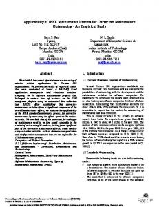
Graph 2. Plot of multistrategy stopping rule for DR5 at a minimum 90% confidence level.
IV. APPLICATIONS AND RESULTS RHS of (31) is the dollar amount of savings due to stoppingaction taken, by not executing the remaining test cases and by not correcting or detecting remaining faults (or branches). LHS of (31) is the dollar amount of potential loss if those remaining faults or coverage were to be corrected after release. If RHS is more than LHS in (31), then, it is a positive gain; otherwise, a negative loss. Let #TC total number of test cases, #NC total number of coverage, and #MC minimum coverage required, which is equal to CL times #NC. Below in Table I are the 6 varying cost-scenarios for Table II that also indicates the subtle effect due to additional information on the range of . There are five quadruplets in Table II, each signifying one data set, where each row in a quadruplet pertains to one of the four sensitivity studies for six cost-scenarios. Note that the first rows in each quadruplet demonstrate a test environment where the #TC is not available with therefore no confidence level (CL) specified. Thus, the testing halts whenever the one-
step-look-ahead formula in (27) holds after at least two test cases with nonzero failures or branch coverage. Second rows in each quadruplet again possess no specified CL, but testing is allowed to continue until or past a certain given minimal number of test cases specified by the analyst and denoted by #TC due to an availability of budget resources, when again (27) is first verified. To exemplify in Table II, for DR5’s first row, stop at second test-case after covering four branches when (27) is first verified. For DR5’s second row, when CL did not apply due to final number of failures or branches unknown, at least a typical prescribed minimal 1094 test cases were allowed to run at which the decisive (27) was also verified. Third and fourth rows in each quadruplet behave with respect to a confidence level of 0.80 (or 80%) and 0.9 (or 90%), respectively. Testing may halt on or after ensuring this specified minimal confidence level of coverage, since the total number of failures or branches is available. #TC in rows 3 and 4 simply display the total prescribed number of test cases for each data set. For DR5s 3rd
˘ S¸AHINOGLU: EMPIRICAL BAYESIAN STOPPING RULE
1435
TABLE I SIX COST SCENARIOS AND THEIR SENSITIVITY STUDIES FOR TABLE II
row, testing stops at 100th test-case for a after cov, which is found by ering 38 branches, exceeding the # # . Also, “a” per undiscovered fault should be at most $26 950 according to the scenario (1), “b” should be at least $17 405 for the scenario (3), and “c” should be at least $15, in order for the stopping rule to be cost effective. due to scenario “(5)Saved” with Total savings is $ the assumed cost parameters as shown in Table II and Screen 1. , one stops at 2042nd test-case For DR5s 4th row, with . covering 42 branches to save The body of test cases is essentially randomized as in the major assumption of Poisson or Bernoulli counting processes. or losses are definitely a function of the cost Savings parameters involved in each scenario. Essentially, if the cost of redeeming coverage (failure or branch) is high, then it is disadvantageous to stop prematurely with respect to a stopping-rule algorithm, such as in MESAT. If the cost parameters are not known, then a sensitivity analysis can be conducted to observe a range of losses or savings. MESAT enjoys the benefit of a confidence level (CL) at will due to budget resources’ availability, in addition to a one-step-ahead-criterion (27) controlled by a divergence factor, “d.” Moreover, the MESAT algorithm effectively accounts for the clumping of the coverage, as well as the positive autocorrelation among the observations in an aggregate. MESAT is also flexible when the final number of coverage may not be known as exemplified in Table II, where you allow a minimal number of test cases to run. This method is also flexible for employing variable cost values, “a”, “b, ” or “c”,, at different test cases across the spectrum, where some test cases may have more weight than others. implies the usage of default Note that in Table II, implies the implemenstandard Beta prior, whereas tation of the generalized Beta prior treated. It is clear that as the economic stopping criterion “d” varies from a liberal (higher) to a conservative (lower) threshold, the stopping rule is shifted and postponed to a later test-case, if not the same. By a conservative set-up, we mean a scenario where the stopping rule is trying not to miss any failures and testing activity is likely to stop later, rather than sooner. The correlation behavior within each clump is represented by our choice of and in the light , like in of previous engineering judgment. Note that for and as imposed in the empirical Bayesian sense in the examples of Table II, the posterior r.v. of displays a distinctly left-skewed behavior. It has been observed that the stopas in e.g., ping occurs earlier in this scenario. However, in , where the Beta distribution looks evenly symmet, the rical as opposed to the presently skewed ones since correlation among coverage in each test-case is not that strong. In the latter case, it has been observed that the stopping rule then
was delayed somewhat if not considerably. Therefore a choice of by Appendix I as in the goodness of fit tests is statistically feasible and acceptable. As for the range of correlation coefficient of LSD, , having a range of first 1.0 (uneducated guess) and then gradually dropping to a 0.5 does generally, if not always, have a subtle savings effect. This is why a Generalized Beta prior [5] was chosen to incorporate the expert opinion for the range of and recognize the infeasibility of very low imposed to lend freedom to versatility rather than assuming the default case of flat when anything goes to avoid statistically unrealistic autocorrelation values of . Note that in Appendix I, the goodness of fit chi-square tests do not involve counts of zero for the underlying LSD tested as the r.v. w for LSD takes as shown in (2) where the on nonzero values, constant “a” is given by (3). Therefore, the blocks will show the frequencies of nonzero entities, where the zero count can be found by subtracting from the total number of test cases for each data set. Screen 1 displays the menu of the aforementioned parameters, including the moving average with a default value of 1 and the goodness of fit test as in Appendix I. It has been found that for DR5, a moving average of 32 gives the best smoothing practice, which in turn calculates the corresponding exponential smoothing factor of 0.0606 [47]. Variable cost data can also be applied, either with a linearly changing slope or by using forced data of the cost parameters c, b, and a, respectively, for each test case entered. V. DISCUSSION AND CONCLUSION The contribution of proposed methodology lies in an empirical Bayesian approach to determine an economically efficient stopping rule in a CP setting that takes the accumulation of failure clumps at each step into account in a software-failure (or branch coverage) counting process. This work is a follow-up to previous research done on Poisson LSD as applied to computer software testing [10]–[13]. This research also presents an alternative to the previous publication in that the compounding distribution was assumed to be geometric (hence, Poisson Geometric) due to its forgetfulness or independence property of the clumped failures and where additionally the stochastic time index was assumed to be in terms of CPU seconds [6]. This paper also addresses the effort-domain problem where the unit tests per calendar weeks are now replaced by test cases or test vectors as sometimes called in embedded-chips testing. However, in this paper, the compounding density is an LSD where failures are interdependent assumed to affect each other adversely by employing test cases as opposed to a continuous time
1436
IEEE TRANSACTIONS ON INSTRUMENTATION AND MEASUREMENT, VOL. 52, NO. 5, OCTOBER 2003
TABLE II STOPPING RULES “S( 1 ) = s” OF DR1(#NC = 134 IN #TC = 200) OF ROWS 1–4, DR2(#NC = 92 IN #TC = 185) OF ROWS 5–8, DR3(#NC = 44 IN #TC = 100) OF ROWS 9–12, DR4(#NC = 63 IN #TC = 200) OF ROWS 13–16, DR5(#NC = 46 IN #TC = 2176) OF ROWS 17–20 WHEN = 8 AND = 2. (3). WITH THE TWO-STAGE APPLICATION, THERE IS ADDITIONAL +$58 000 FOR DR5 AS CALCULATED IN TABLE VI. ALL OF TABLE II’S STOPPING RULES SHOWN ARE ONE-STAGE TESTING RESULTS FOR SIMPLICITY PURPOSES
TABLE III STOPPING RULES USED IN CASE STUDY [49]
domain in terms of CPU seconds or hours or weeks. Recall that the dual of a time-dependent Poisson process is a time-independent discrete Bernoulli process whose theory is sufficiently strong to handle the unit test-case phenomenon replacing the unit test-week as a stochastic index where the response variable is the number of failures or branch coverage etc. [20]. This is in line with the test-case based testing activity, where limiting distribution of the sum of the nonhomogeneous Bernoulli variables process, where np, with n number of is the Poisson Bernoulli trials and p probability of detecting a failure or covering a branch ([9] and [50], p. 304). The stopping rule is applied to five effort-domain test data sets, namely DR1 to DR5 compiled by CS Labs at Colorado State University [17]–[19], [48], [49] and also to a DoD data set [41], [44]. This stopping-rule method is a new derivative of the original publications on “The Compound Poisson Reliability
Model” [11], [12]. The number of failures or branches covered is independent from test-case to test-case. Test cases are randomized, and not in any specific order. However, the total number of contributions or coverage at each one-step-look-ahead check assures the testing activity to stop due to a specified criterion “d” for a set of specified cost parameters and imposed on the data set itself having learned from previous similar activity or subjective guesswork. Then, the software analyst can apply a subsequent testing strategy after stopping due to saturation effect with respect to an economic criterion, provided that a desired confidence level is satisfied in order to see the effect of the following scheme. Therefore, the same algorithm can be applied for a next strategy to judge where to stop. Hence a mixed sequence of strategies can be employed for best efficiency to save time and effort, i.e., overall resources. This is sometimes called “mixed strategy testing” [17]–[19], [41], [44]. It is shown by McDaid and Wilson [38] that two stage sampling is superior to single stage as illustrated in our examples given in Screen 1 and Graphs 1 and 2. It is most likely that by sacrificing only small percentage of failure or branch coverage accuracy, one can literally spare wasted testing resources because of persisting on the same futile testing strategy, on a journey to the unknown. Also, as “d” gets smaller, usually stopping is delayed for fine-tuning. The saving of testing resources can be considerably crucial for large testing problems. This stopping-rule method is therefore based on a Bayesian approach of updating the historical information experienced for future LSD (negative decision-making. It assumes by Poisson
˘ S¸AHINOGLU: EMPIRICAL BAYESIAN STOPPING RULE
binomial, for a special case) model where the contributed failure or branch coverage clumped in a test-case is positively correlated. This implies that an occurrence of failure or branch is likely to invite a next failure or branch. For further research, a variety of informative priors can be considered as alternatives for [5], [21]. to conjugate prior generalized Beta Further, to provide readers with fundamental information about what sorts of methods currently exist for a variety of projects as listed in Table III for the stopping-rule problem this paper is dealing with, and to provide evidence that the method proposed herein is a substantial improvement, lists of comparisons over the other existing methods in circulation are presented in Appendix II. In summary, the proposed MESAT is progressive and more data friendly in terms of its EDA that other methods do not attempt to study for diagnosis. MESAT is suitable for those data sets, which satisfy the goodness of fit criterion of their clump-size distribution with respect to a hypothesized LSD. This property of MESAT is therefore discriminative, rather than fitting for all purposes. It is generally true that the branch coverage data sets obey the assumptions stated at least in this paper. This is why five out of five data sets proved positive for the LSD assumed; hence good fits are declared for NBD in natural consequence by (1) to (13) in Section II. MESATs only seemingly subtle disadvantage is the assumption of independent (randomized) test cases, which is a requirement for the independent increments property of the Poisson processes as the major underlying distribution of counts in this research. However, as earlier explained in Section I, the randomization assumption is a practical reality in testing practice. Even if otherwise suspected, there is no universally accepted solution of modeling the correlation of test cases for each testing activity whose results are not known in advance by the nature of surprise factor in software testing. APPENDIX I
1437
1438
IEEE TRANSACTIONS ON INSTRUMENTATION AND MEASUREMENT, VOL. 52, NO. 5, OCTOBER 2003
process of HDL verification, we first need to create failures as interruptions, where an interruption is an incident where one or more new part of the model are exercised. Using branch coverage as a test criterion, an interruption, therefore indicates one or more new branches are covered. We set a probability for the interruption rate B and choose an upper-bound level of confidence C. Experimentally, we do not examine the hypothesis unless the interruption rate becomes smaller than the preset value B. When so, we calculate the number of test patterns needed to have at least C confidence of not having any new branch in the next N patterns and run them. If an interruption occurs, we continue examining the hypothesis until we prove it and then stop. In this approach, we assume that coverage items, or indeed interruptions are independent and have equal probabilities of being covered. The rate of interruption is decreasing and we assume no interruptions will occur in the next N test cases; then, the expected probability of interruptions will be [27], [28], [34]
APPENDIX II COMPARISONS OF THE PROPOSED CP RULE WITH OTHER STOPPING RULES Almost all of the existing statistical models used to determine stopping-points stem from research results in software engineering [22], [34], [37]–[41], [44]. Many models have been proposed assessing the reliability measurements of software systems to help designers evaluate, predict, and improve the quality of their software systems [23]–[32]. However, software reliability models aim at estimating the remaining faults in a given software program, which makes the direct use of such models not beneficial in estimating the number of remaining uncovered branches in a behavioral model since the remaining uncovered branches are known. Instead, the estimation process can be slightly modified to focus on the expected number of faults, or coverage items in the case of behavioral model verification, within the next unit of testing time. Unfortunately, all the existing software reliability models assume that failures occur one at a time, except for the proposed MESAT approach that uses a CP. Based on this assumption, expectations of the times between failures are carried on. In observing new coverage items in a behavioral model, branches are typically covered in clumps. Besides, in the proposed MESAT tool, the positive correlation within a clump is taken into account. The confidence-based modeling approach [27], [28] takes advantage of hypothesis testing in determining the saturation of the software failure. A null hypothesis H is performed and later examined experimentally based on an assumed probability distribution for the number of failures in a given software. Suppose that a failure has a probability less than or equal to B to occur, B confident that H is true. Similarly, then we are at least if the failures for the next period of testing time have the same probability of at least B to occur, then for the next N testing cycles, we have a confidence of at least C that no failures will happen, where C
B
(A2.1) (A2.2)
, then by using (A2.2), . This is a If single-equation stopping-rule method, which can be likened to a parallel system of N independent components whose reliabilito satisfy an overall network ties are identical to be each reliability of C ([36], p. 265). To apply Howden’s model to the
(A2.3) where T is the last checked point in testing, and this leads to the reformulation of (A2.1) as follows: N C
(A2.4)
Branches in behavioral models are usually covered in clumps during the verification process. One could consider the event of having one or more new covered branches as an interruption. Thus, interruptions could be treated as failures with a chosen upper-bound probability B where the hypothesis is not examined unless the interruption rate becomes smaller than this preset value B. The confidence of having an interruption is then calculated based on the interruption rate. Nevertheless, it was assumed that interruptions are independent of each other. Some authors support that this is not correct [33], [34]. In fact, branches in behavioral models can be classified as dominant, and controlled branches where it is impossible to cover the lower level branches without covering their dominant branches. Moreover, the sizes of the interruptions are not modeled in [27], [28] making the understanding of the branch behavior less informative. Sanping Chen and Shirley Mills developed a statistical Markov process or Binary Markov model [29], [34] where the probabilistic distribution assumptions are the same as confidence-based model except that failures are statistically dependent with a certain unknown correlation constant, . Again, if interruptions are correlated, then the probability of having no interruptions in the next N test cases is p
N B
B
B
N
(A2.5)
p N B . Chen and that makes the confidence as C Mill’s model still doesn’t deal with the issue of clumping. Furthermore, the value of in this model is unknown, and authors experimentally assumed different values ranging from 0 to 0.9 and obtained different results. Thus, needs to be determined experimentally. In Howden’s model, the assumption that failures or interruptions have a given probability B independently is erroneous.
˘ S¸AHINOGLU: EMPIRICAL BAYESIAN STOPPING RULE
1439
TABLE IV RESULTS OF STOPPING-RULE COVERAGE FOR STATIC CASE STUDY WHERE COVERAGE PER TESTING PATTERN CAN BE CALCULATED (i.e., COVERAGE/PATTERNS) WITHOUT USING COST FACTORS [49]
Branches in an HDL model, as we know are strongly dependent of each other. In fact, we can classify some branches where it is impossible to cover the lower level ones without covering their dominants. Moreover, the clump sizes caused by the interruptions are not modeled in this study making the decision of continuing or stopping the testing process inaccurate. Last, this work does not incorporate the cost of testing or releasing the product, and the goal of testing in the first place is not only having a high quality product but also minimizing the testing costs [34]. Dallal and Mallows [1] assumed that the total number of failures in a given software is a random variable with unknown mean, and the number of failures occur during the testing time is a nonhomogeneous Poisson process with increments g t . The time needed for a single failure to occur is distributed as g t , which can be assumed exponential. This model has a better description for the failure process over the previous models so far discussed, such as Howden and modified Howden’s in Chen and Mill’s models. However, it still suffers from the problem of not having more than one interruption at a time, which reduces the efficiency of the model when applying it to branch coverage estimation [34]. Finally, the author of this manuscript, S¸ahino˘glu et al. [11]–[13], [17]–[19] whereas applied a CP model that models the branch coverage process of VHDL circuits utilizing the benefits of the “Dallal and Mallows” economic model by reformulating it [6] and solving the clumping phenomenon of branches being covered in the testing process. This model uses the empirical Bayesian principles for the compounded
Poisson counting process. It was previously introduced as a software reliability model for the remaining number of failures’ estimation in 1992 [11] and later modified to incorporate a version of the cost modeling proposed by Dallal and Mallows in 1995 [6], [13]. Recently, it was formulated to model the branch coverage process in behavioral models [17]–[19]. The idea is to compound potentially two probability distributions, for both the number of interruptions and the size of interruptions. The resulting compound distribution is assumed to be the probability distribution function of the total number of failures, or coverage items, at a certain testing time point. The parameters of the distributions are also assumed to be random variables based on the empirical Bayesian estimation. For modeling the branch coverage process for behavioral models, it is assumed that the number of interruptions over the time, N t , is a Poisson process with mean , and the size of each given interruption, w , is distributed as a Logarithmic Series Distribution (LSD). See diagnostics of Appendix I for the justification of LSD of clump sizes. The resulting compound distribution for the total number of failures, which is the sum of the sizes, is also known as an . The NBD, if the Poisson parameter is set to k CP model takes into account the clumps of the coverage items in a statistical manner by updating the assumed probability distribution parameters in every test-case based on the testing history. However, interruptions in the testing process are assumed to be independent, mainly due to the “independent increments property” of the anchoring Poisson process. The proposed MESAT also incorporates a minimal confidence rule
1440
IEEE TRANSACTIONS ON INSTRUMENTATION AND MEASUREMENT, VOL. 52, NO. 5, OCTOBER 2003
TABLE V RESULTS OF COST ANALYSIS FOR A DYNAMIC CASE STUDY WHERE a = $5000; b = $500, AND c = $1 [44]
in addition to applying the one-step-ahead formula of (27) for assessing whether to stop or continue economically. All the previously discussed stopping rules assume that the failures or interruptions are random processes according to a given probability distribution. A sequential sampling technique that doesn’t involve any assumptions on the probability distributions for the failure process was presented in [25]. Recently, the technique is applied to VHDL models in determining the stopping points for a given testing history of branch coverage [30]. The model evaluates the stopping decision based on three key , the supplier risk , and factors: the discrimination ratio . If the number of cumulative coverage at the consumer risk time t is X t , then the testing process should be stopped at Xt
(A2.6)
The stopping decision strongly depends on the value of much more than and . The decision doesn’t incorporate any cost model of the testing process. In [25], the variable was modified with respect to testing strategies such that if higher coverage were achieved in the previous test strategy, the value of is increased in the current test strategy in order to decrease the expectation of achieving more coverage in the current strategy. The
new value of , therefore, becomes: , where is the coverage increase achieved in the previous test strategy The . This type of stavalue of , however, remains the same if tistical modeling doesn’t use any priori probability distribution for the data provided. This is one reason why the sequential sampling models are widely used in many testing areas [33], [34]. However, the cost of testing is not modeled in making the stopping decision. Moreover in the opinion of this manuscript’s author, the stopping point determined by the sequential sampling model is very sensitive to the value chosen during the testing process. (A2.6) is an equation subject to an abusive use for purposes of experimental validation. Authors of this approach [30] have earlier suggested values for up to 250, whereas Musa’s [25] text only uses in the order of 5 or 10. Excessive values of pose a contradiction and threat to the Wald’s SPRT theory for sequential testing in terms of type I (whose probability is ) and II (whose probability is ) errors. The same holds true for which authors in their related paper have suggested to be , a relatively exaggerated value compared to Musa’s . Singpurwalla et al. [37], [40], [45], McDaid and Wilson [38] and Ross [39] have developed their own stopping rules with differing statistical assumptions on one- or two-stage testing schemes. However, because these techniques have not been experimented on “hardware or silicon testing” with respect
˘ S¸AHINOGLU: EMPIRICAL BAYESIAN STOPPING RULE
1441
TABLE VI RESULTS OF DR5 MIXED STRATEGY STOPPING- RULE AT A MINIMUM 80% CONFIDENCE LEVEL
to branch coverage, no comparative results are available in the engineering literature in terms of merits. The above arguments suggest that the proposed MESAT employing both a minimal confidence rule and one-step-look-ahead formula within a single or multistage testing scenario to justify a decision taken whether to continue or stop testing, has the imminent advantages of recognizing the clumping effect in coverage testing as well as incorporating the economic criteria in addition to its data discriminative traits by conducting EDA through diagnostic checks. It is imperative that a diagnostic check, such as in Appendix I, be undertaken if similar exhaustive test results are available. This is necessary to justify the usage of the LSD model for the clump sizes, a model that eventually leads to the NBD assumption for the total number of coverage by default in the wake of the expression assumed to hold true.
For a more thorough comparative case study, research done by Hajjar and Chen was utilized [22], [49], where nine different stopping rules, shown in Table III were applied to 14 different VHDL models [44]. The results of the stopping-rule determinations are shown in Table IV, including results without the use of any stopping rule. This stopping-rule comparison portrays the CP method as having one of the lowest efficiencies based on a naive “coverage per testing pattern” index, which is defined as the number of branches covered divided by the total test patterns used. Despite their index rating, CP found the most faults for 10 out of the 14 VHDL models, while ranking second in B15, third in B01 and fourth in B04. Furthermore, no economic analysis has been performed to illustrate the monetary gain or loss associated with the various stopping rules. Let us now use the cost benefit criterion of (31) in the main paper, where RF is the remaining number of failures uncovered and RT is the remaining
1442
IEEE TRANSACTIONS ON INSTRUMENTATION AND MEASUREMENT, VOL. 52, NO. 5, OCTOBER 2003
RESULTS
OF
TABLE VII DR5 MIXED STRATEGY STOPPING RULE 90% CONFIDENCE LEVEL
ACKNOWLEDGMENT AT A
MINIMUM
number of test patterns unused when stopped. For an example, since cost of redempwe will use tion of after-market is 10 times more than that of before. Using the Sys7 data with CP, we get [44], [48]:
tive by DB, we get
, showing CP to be cost effec. Comparing Sys7 with
, showing DB to not . Why a be cost effective by ratio of 10 used between before-release and after-release costs? The main reason is that silicon testing, unlike software testing, is more expensive for uncovered branches or failures. Tables VI and VII illustrate the results of a mixed-strategy testing activity. Although access to the VHDL model data used in Hajjar et al.’s research [49] was not available, a cost analysis could still be applied to their results. By performing this cost analysis on the stopping points in Table III and comparing the results, the economically beneficial stopping rules were determined for a given cost criterion. Using the cost criterion of (31), in a case study in which a cost index was applied to the data with cost , and . The CP stopping values of rule was clearly more beneficial. As can be seen in Table V, of the nine stopping rules used in that study, the CP stopping rule ranked very high with regards to savings in many of the VHDL data sets used for comparison. Low cost of testing in conjunction with high post-release repair cost render the CP stopping rule superior to many of the other stopping rules in the study. The incentive behind the mixed strategy testing is that a bug undetected in a silicon embedded chip is much more costly than a bug in software, and, therefore, the stopping rule needs to be very conservative. At the end of the spectrum, because the cost of testing is much less than the cost of a bug in silicon, it seems that a nonconservative stopping rule is worse than some other rules. Another angle can be extracted from the Table IV, where the number of branch coverage in SB (Hajjar and Chen’s proposed rule) is more than 10% fewer than the original (no stopping rule). This is probably not acceptable in hardware. A comparison: ATPG typically aims for % fault coverage, and a user would probably aim for even 1% increases in coverage point, if it is achievable in a reasonable amount of computation. So the proposed rule is probably a good rule to “switch” instead of “stop” the testing process.
The author would like to thank Prof. A. S. Al-Khalidi, from Texas A&M University’s Institute of Statistics and formerly a Senior Faculty Member at Dokuz Eylul University’s Department of Statistics, Izmir, Turkey, for his earlier theoretical contributions as cited. The author would also like thank J. Larson and M. Hicks for expert java programming, as well as the two distinguished Guest Editors of the Special Section on Testing of the IEEE Instrumentation and Measurement Society, for their time and effort, and the Instrumentation and Measurement Transactions Administrator for his assistance. REFERENCES [1] S. R. Dallal and C. L. Mallows, “When should one stop testing software,” J. Amer. Stat. Assoc., vol. 83, pp. 872–679, 1988. [2] M. H. DeGroot, Optimal Statistical Decisions. New York: Mc GrawHill, 1970. [3] N. Johnson, S. Kotz, and J. Kemp, Univariate Discrete Distributions, 2nd ed. New York: Wiley, 1993. [4] S. Kotz et al., Encyclopedia Stat. Sciences, 1988. Vol. 5, 11–113; Vol. 6, 169–176. [5] T. G. Pham and N. Turkkan, “Bayes binomial sampling by attributes with a generalized-beta prior distribution,” IEEE Trans. Rel., vol. 41, pp. 310–316, Mar. 1992. [6] P. Randolph and M. S¸ahino˘glu, “A stopping-rule for a compound Poisson random variable,” Appl. Stochastic Models Data Anal., vol. 11, pp. 135–143, June 1995. [7] S. Samuels, Handbook of Sequential Analysis, B. K. Ghosh and P. K. Sen, Eds. New York: Marcel Dekker, 1991, ch. 16, pp. 381–405. [8] C. C. Sherbrooke, Discrete Compound Poisson Processes and Tables of the Geometric Poisson Distribution. Santa Monica, CA: Memorandum RM-4831-PR, The Rand Cooperation, July 1966. [9] M. S¸ahino˘glu, “The limit of sum of Markov Bernoulli variables in system reliability evaluation,” IEEE Trans. Rel., vol. 39, pp. 46–50, Apr. 1990. [10] , “Negative binomial density of the software failure count,” in Proc. 5th Int. Symp. Computer and Information Sciences (ISCIS), vol. 1, Oct. 1990, pp. 231–239. [11] , “Compound Poisson software reliability model,” IEEE Trans. Software Eng., vol. 18, pp. 624–630, July 1992. [12] M. S¸ahino˘glu and U. Can, “Alternative parameter estimation methods for the compound Poisson software reliability model with clustered failure data,” Software Testing Verification Rel., vol. 7, pp. 35–57, Mar. 1997. [13] M. S¸ahino˘glu and A. S. Al-Khalidi, “A Bayesian stopping-rule for software reliability,” in Proc. 5th World Meeting ISBA, Satellite Meeting to ISI-1997, Aug. 1997. [14] M. S¸ahino˘glu, J. J. Deely, and S. Capar, “Stochastic Bayes measures to compare forecast accuracy of software-reliability models,” IEEE Trans. Rel., pp. 92–97, Mar. 2001. [15] N. Johnson, S. Kotz, and N. Balakrishnan, Continuous Univariate Distributions, 2nd ed., 1995, vol. 2. [16] G. G. Roussas, A First Course in Mathematical Statistics. Reading, MA: Addison-Wesley, 1973, p. 253. [17] T. Chen, M. S¸ahino˘glu, A. von Mayrhauser, A. Hajjar, and C. Anderson, “How much testing is enough? Applying stopping-rules to behavioral model testing,” in Proc. 4th Int. High-Assurance Systems Engineering Symposium (HASE), Nov. 17–19, 1999, pp. 249–256. [18] M. S¸ahino˘glu, A. von Mayrhauser, A. Hajjar, T. Chen, and Ch. Anderson, “On the efficiency of a compound Poisson stopping-rule for mixed strategy testing,” in Proc. IEEE Aerospace Conf., Aspen, CO, Mar. 6–13, 1999. [19] T. Chen, M. S¸ahino˘glu, A. von Mayrhauser, A. Hajjar, and C. Anderson, “Achieving the quality of verification for behavioral models with minimum effort,” in Proc. 1st Int. Symp. Quality Electronic Design (ISQED), San Jose, CA, Mar. 20–22, 2000, pp. 234–239. [20] E. Çınlar, Introduction to Stochastic Processes. Englewood Cliffs, NJ: Prentice-Hall, 1975. [21] M. S¸ahino˘glu and A. Al-Khalidi, “A stopping-rule for time-domain software testing,” in Proc. 10th Int. Symp. Software Reliability Engineering, Boca Raton, FL, Nov. 1–4, 1999.
˘ S¸AHINOGLU: EMPIRICAL BAYESIAN STOPPING RULE
[22] A. Hajjar and T. Chen, “A new stopping-rule for behavioral model verification based on statistical Bayesian technique,” IEEE Trans. Computer-Aided Design, to be published. [23] S. Gokhale and K. Trivedi, “Log-logistic software reliability growth model,” Proc. 3rd IEEE Int. High Assurance Systems Engineering Symp. (HASE), pp. 34–41, Nov. 1998. [24] A. Goel, “Software reliability models: Assumptions, limitations, and applicability,” Software Eng., vol. SE-11, no. 12, pp. 1411–1423, Dec. 1985. [25] J. Musa, “A theory of software reliability and its application,” Software Eng., vol. SE-1, no. 3, pp. 312–27, 1975. [26] D. Mills, “On the statistical validation of computer programs,” IBM FSD, Rep. FSC-72-6015, 1972. [27] W. Howden, “Confidence-based reliability and statistical coverage estimation,” Proc. Int. Symp. Software Reliability Engineering, pp. 283–291, Nov. 1997. , “Systems testing and statistical test data coverage,” in Proc. [28] COMPSAC, Aug. 1997, pp. 500–505. [29] S. Chen and S. Mills, “A binary Markov process model for random testing,” Software Eng., vol. 22, no. 3, pp. 218–223, 1996. [30] T. Chen, I. Munn, A. von Mayrhauser, and A. Hajjar, “Efficient verification of behavioral models using the sequential sampling technique,” in Proc. Symp. Very Large Scale Integration, Brazil, 1999. [31] B. Barrera, “Code coverage analysis-essential to a safe design,” Electron. Eng., pp. 41–44, Nov. 1998. [32] B. Dickinson and S. Shaw, “Software techniques applied to VHDL design,” New Electron., no. 9, pp. 63–65, May 1995. [33] A. Hajjar, T. Chen, and A. von Mayrhauser, “On statistical behavior of branch coverage in testing behavioral VHDL models,” in Proc. IEEE High Level Design Validation and Test Workshop, Berkeley, CA, Nov. 2000. [34] A. Hajjar, T. Chen, I. Munn, A. Andrews, and M. Bjorkman, “Stopping criteria comparison: Toward high quality behavioral verification,” in Proc. Int. Symp. Quality in Electronic Design, San Jose, CA, Mar. 2001. [35] G. G. Roussas, A First Course in Mathematical Statistics, 1st ed. Reading, MA: Addison-Wesley, 1973. [36] E. E. Lewis, Introduction to Reliability Engineering, 2nd ed. New York: Wiley. [37] E. H. Forman and N. D. Singpurwalla, “An empirical stopping rule for debugging and testing computer software,” J. Amer. Stat. Assoc., vol. 72, pp. 750–757, 1977. [38] K. McDaid and S. P. Wilson, “Deciding how long to test software,” The Statistician, vol. 50, pp. 117–134, 2001. [39] S. M. Ross, “Software reliability: The stopping rule problem,” IEEE Trans. Software Eng., vol. 11, pp. 1472–1476, 1985. [40] N. D. Singpurwalla, “Determining an optimal time interval for testing and debugging software,” IEEE Trans. Software Eng., vol. 17, pp. 313–319, 1991. [41] M. S¸ahino˘glu, C. Bayrak, and T. Cummings, “High assurance software testing in business and DoD,” Trans. Soc. Design Process Sci., vol. 6, no. 2, pp. 107–114, 2002. [42] K. Abdullah, J. Kimble, and L. White, “Correcting for unreliable regression integration testing,” in Proc. Int. Conf. Software Maintenance, Nice, France, Oct. 1995, pp. 232–241. [43] W. Notz, private communication, Aug. 2002. [44] M. Hicks, “A Stopping Rule Tool for Software Testing,” M.S. thesis, Dept. Comput. Inform. Sci., Troy State Univ., Montgomery, AL, Dec. 2000.
1443
[45] N. D. Singpurwalla and S. P. Wilson, Statistical Methods in Software Engineering. New York: Springer, 1999. [46] M. S¸ahino˘glu and E. H. Spafford, “A Bayes sequential statistical procedure for approving products in mutation-based software testing,” in Proc. IFIP Conf. Approving Software Products (ASP), Germany, Sept. 17–19, 1990, pp. 43–56. [47] D. Anderson, D. J. Sweeney, and T. A. Williams, An Introduction to Management Science—Quantitative Approaches to Decision Making, pp. 735–743, 2002. [48] M. S¸ahino˘glu and S. Glover, “Economic analysis of a stopping rule in branch coverage testing,” in Proc. 3rd Int. Symp. Quality Electronic Design, San Jose, CA, Mar. 18–21, 2002, pp. 341–346. [49] A. Hajjar and T. Chen, “Improving the efficiency and quality of simulation-based behavioral model verification using dynamic Bayesian criteriaxc,” in Proc. 3rd Int. Symp. Quality Electronic Design, San Jose, CA, Mar. 18, 2002, pp. 304–309. [50] K. S. Trivedi, Probability and Statistics with Reliability, Queuing and Computer Science Applications, 2nd ed. New York: Wiley, 2002. [51] S. R. Das, C. V. Ramamoorthy, M. H. Assaf, E. M. Petriu, and W.-B. Jone, “Fault tolerance in sytems design in VSLI using data compression under constraints of failure probabilities,” IEEE Trans. Instrum. Meas., vol. 50, pp. 1725–1745, Dec. 2001.
Mehmet S¸ahino˘glu (S’78–M’81–SM’93) received the B.S. degree in electrical and computer engineering from the Middle East Technical University (METU), Ankara, Turkey, in 1973, the M.S. degree in electrical and computer engineering from the University of Manchester Institute of Science and Technology, Manchester, U.K., in 1975, and the Ph.D. degree in both electrical and computer engineering and statistics from Texas A&M University, College Station, in 1981. Prior to joining the CIS Department, Troy State University, Montgomery, AL, as its first Eminent Scholar and Chairman in 1999, he was at METU for 20 years as a Reliability Consultant to the Turkish Electricity Authorities (TEK) and The National Defense Industry, Ankara, from 1976 to 1992, as a Professional Certified Engineer. He then served for five years as a Founder Dean of Science and Founder Chairman of the Department of Statistics at Dokuz Eylul University, Izmir, Turkey, from 1992 to 1997. He taught at Purdue University, West Lafayette, IN, from 1989 to 1990 and 1997 to 1998, and Case Western Reserve University, Cleveland, OH, from 1998 to 1999 as a Visiting Fullbright and NATO Research Scholar, respectively. He retired in 2000 after 26 years of civil service in Turkey as a Professor Emeritus. He published in electric power earlier in his career, and computer software reliability and testing in later years. He is accredited with the original findings of the “Compound Poisson Software Reliability Model” to account for the multiple (clumped) failures in predicting the total number of failures at the end of a mission time, and the “MESAT: Compound Poisson Stopping Rule Algorithm” in software testing literature. He is also jointly responsible, with Dr. David L. Libby, for the original derivation of the “Forced Outage Ratio (FOR)” or “Generalized Three-Parameter Beta (G3B)” pdf. He recently created an Exact Reliability Block Diagram Calculation (ERBDC) Tool, which is a novel graphical technique in the literature for quantifying and designing the reliability of computationally complex systems. Dr. S¸ahino˘glu is a Fellow of the Austin-based Society of Design and Process Science and a member of ACM, AFCEA, ASA, and an elected member of ISI.