An Empirical Comparison of Affine and Non-Affine ... - Semantic Scholar

An Empirical Comparison of Affine and Non-Affine Models for Equity Index Options Peter Christoffersen Kris Jacobs Karim Mimouni Faculty of Management, McGill University∗ January 25, 2006

Abstract The existing literature on equity index option valuation largely focuses on affine models because they lead to closed-form solutions for option prices. This paper investigates the empirical shortcomings associated with affine models, using data on S&P500 call options. We find that the root mean squared dollar error for a simple non-affine continuous-time stochastic volatility model is 25-27% lower than that of the benchmark continuous-time affine stochastic volatility model in- and out-of-sample. The analytical convenience of affine option valuation models therefore comes at a price, and non-affine models ought to be investigated more extensively. We also compare the empirical performance of affine and non-affine discrete-time models. While the performance of the discrete-time non-affine model is similar to that of the continuous-time non-affine model, the discrete-time affine model outperforms the continuous-time affine model. We provide some intuition for these findings. At the methodological level, our analysis uses a novel technique based on the Auxiliary Particle Filter. This technique allows for an analysis of option valuation models using options data that imposes consistency with underlying equity returns. It is straightforward to implement and it can be used in a variety of applications and on various loss functions. JEL Classification: G12 Keywords: Stochastic volatility; GARCH; option valuation; particle filtering. ∗

Christoffersen and Jacobs are also affiliated with CIRANO and CIREQ and want to thank FQRSC, IFM2 and

SSHRC for financial support. Mimouni was supported by IFM2 . We thank seminar participants at American University, Case Western Reserve, Northwestern, Rice University, SBFSIF, and the University of Calgary, and in particular Torben Andersen, Alex David, Vadim di Pietro, Jin Duan, Jeff Fleming, Anurag Gupta, Michael Johannes, Nour Meddahi, Barbara Ostdiek, Brad Paye, Marcel Rindisbacher, Peter Ritchken, and Neal Stoughton for helpful comments. Any remaining inadequacies are ours alone. Correspondence to: Peter Christoffersen, Faculty of Management, McGill University, 1001 Sherbrooke Street West, Montreal, Quebec, Canada, H3A 1G5; Tel: (514) 398-2869; Fax: (514) 398-3876; E-mail: peter.christoff[email protected].

1

1

Introduction

Following the finding that Black-Scholes (1973) model prices systematically differ from market prices, the literature on option valuation has formulated a number of theoretical models designed to capture these empirical biases. One particularly popular modeling approach has attempted to correct the Black-Scholes biases by modifying the assumption that volatility is constant across maturity and moneyness. Estimates from returns data and options data indicate that return volatility is time-varying, and modeling volatility clustering leads to significant improvements in the performance of option pricing models. It has also been demonstrated that it is necessary to model a leverage effect. The leverage effect captures the negative correlation between returns and volatility, and thus generates negative skewness in the distribution of the underlying asset return.1 The existing literature has almost exclusively modeled volatility clustering and the leverage effect within an affine structure.

Affine models of option valuation are convenient because they

lead to closed-form solutions for prices of European equity options. In particular, the affine Heston (1993) model, which accounts for time-varying volatility and a leverage effect, has been implemented in a large number of empirical studies. In order to address the limitations of the affine structure, the Heston (1993) model is often combined with models of jumps in returns and/or volatility.2 However, relatively little is known about the empirical biases that result from imposing the affine structure.3 The existing literature has also almost exclusively modeled volatility clustering and the leverage effect using continuous-time stochastic volatility models. There exists a small discrete-time literature on option valuation using GARCH processes, and in this literature the distinction between affine and non-affine models is also relevant. The affine GARCH dynamic in Heston and Nandi (2000) yields a closed-form solution for option prices, but the extensive empirical literature on GARCH processes that concerns itself with fitting and predicting return volatility almost exclusively uses non-affine processes.4 A small number of studies investigate option valuation assuming 1

The leverage effect was first characterized in Black (1976). For empirical studies that emphasize the importance

of volatility clustering and the leverage effect for option valuation see among others Benzoni (2002), Chernov and Ghysels (2000), Eraker (2004), Heston and Nandi (2000), Nandi (1998) and Pan (2002). 2 For empirical studies that implement the Heston (1993) model by itself or in combination with different types of jump processes, see for example Andersen, Benzoni and Lund (2002), Bakshi, Cao and Chen (1997), Bates (1996, 2000), Benzoni (2002), Chernov and Ghysels (2000), Huang and Wu (2004), Pan (2002), Eraker (2004) and Eraker, Johannes and Polson (2003). 3 Jones (2003) and Benzoni (2002) are notable exceptions that investigate non-affine option valuation models. The non-affine model in Benzoni (2002) does not improve on the performance of the Heston (1993) model, while a number of specification tests in Jones (2003) favor the non-affine constant elasticity of substitution model over the Heston (1993) model. 4 The literature on GARCH processes is too voluminous to cite in full here. The classical references are Engle (1982) and Bollerslev (1986). See Bollerslev, Chou and Kroner (1992) and Diebold and Lopez (1995) for reviews.

2

non-affine GARCH processes for the underlying securities.5 This paper investigates the empirical implications of adopting an affine framework for option valuation. We compare the empirical performance of the affine Heston (1993) stochastic volatility model (AF-SV) with that of a simple non-affine stochastic volatility model (NA-SV). We estimate model parameters using a rich data set of options recorded across time, moneyness and maturity in a framework that imposes consistency with the underlying equity returns. We conduct this empirical analysis using a novel setup that uses the Auxiliary Particle Filter algorithm.

This

methodology provides a convenient filtering algorithm for latent factor models such as stochastic volatility models. Our new methodology is easy to implement, and it can be adapted to provide the best possible fit to the objective function of interest. We also compare the empirical performance of the affine Heston and Nandi (2000) model (AF-GARCH) with that of the non-affine GARCH model (NA-GARCH) of Engle and Ng (1993). We find that the affine framework is very restrictive. We conduct three in-sample exercises and three out-of-sample exercises, and despite the fact that both the AF-SV and the NA-SV models show signs of misspecification, the NA-SV model outperforms the Heston (1993) AF-SV model in all of these exercises. The NA-SV model also outperforms the AF-SV model for all moneyness and maturity categories. On average, the dollar root mean-squared error (RMSE) of the NA-SV we investigate is approximately 25.5% lower than that of the AF-SV model in-sample, and the outof-sample dollar RMSE is 27.5% lower. We therefore conclude that while the closed-form solution provided by affine models is convenient, this analytical convenience comes at a price, and non-affine models need to be studied more extensively. Interestingly, the differences in RMSE between the non-affine discrete-time model (NA-GARCH) and the affine discrete-time model (AF-GARCH) are smaller than in the continuous-time case, approximately 10% in-sample and 15% out-of-sample.6 This finding naturally raises important questions about the relationship between the empirical performance of discrete-time and continuoustime models. Our findings on this issue are perhaps less straightforward to interpret than those on the implications of the affine structure, but we are able to draw a number of important conclusions. The literature contains a number of limit results relating certain classes of discrete-time and continuous-time models.7 Some researchers have interpreted these limit results as evidence that the performance of discrete-time and continuous-time models ought to be very similar when the continuous-time dynamic is the limit of the discrete-time dynamic. This interpretation is somewhat contentious, because a given discrete-time model can have several continuous-time limits, and a 5

See Amin and Ng (1993), Bollen and Rasiel (2003), Bollerslev and Mikkelsen (1996), Christoffersen and Jacobs

(2004a), Duan, Ritchken and Sun (2002), Engle and Mustafa (1992), and Heston and Nandi (2000). 6 See Hsieh and Ritchken (2000) for a related comparison. 7 See for example Duan (1997), Heston and Nandi (2000), Nelson (1990), and Ritchken and Trevor (1999).

3

given continuous-time model can be the limit for more than one discrete-time model.8 While limit results are therefore theoretically intriguing, in some cases their practical relevance may be limited. We find some very interesting differences in the empirical performance of models that are often thought of as equivalent. Most importantly, the AF-SV Heston (1993) model, which is the benchmark model in the continuous-time stochastic volatility literature, significantly underperforms the AF-GARCH Heston-Nandi (2000) model. This result is perhaps surprising, because Heston and Nandi (2000) demonstrate that a restricted Heston (1993) model can be seen as the limit of the AF-GARCH model, but the key is of course that this particular limit is just one of the many available. Which limit obtains depends on the particular mathematical construction used. This finding does not mean that discrete-time GARCH models outperform continuous-time stochastic volatility models. Indeed, the performance of the non-affine NA-GARCH discrete time model of Engle and Ng (1993) is very similar to but slightly worse than the performance of the NA-SV model we investigate. These findings demonstrate that it is difficult to make general statements about discrete-time and continuous-time models. Certain stylized facts may be more conveniently captured by specific continuous-time models, while others are more easily modeled using a particular discrete-time model. This paper merely provides a start to that discussion by documenting the empirical performance of some important benchmark models. After documenting that the benchmark AF-SV Heston (1993) model somewhat surprisingly underperforms relative to a the related AF-GARCH discrete-time model, we proceed by suggesting an aspect of the model that may cause the underperformance. One final remark is in order. Traditionally, the existence of multiple limits has not been the only issue that complicated a comparison of discrete-time and continuous-time models. The two classes of models are typically implemented using very different econometric methods, which renders fair comparisons difficult. Our use of the Auxiliary Particle Filter algorithm9 allows for straightforward comparisons of latent factor volatility continuous time models with discrete time GARCH models, because each model is implemented using the same objective function and the same information set. The novel estimation setup in this paper therefore facilitates comparisons between different classes of models. The paper proceeds as follows. In Section 2 we introduce and discuss the affine and nonaffine continuous-time and discrete-time volatility models. In Section 3 we explain our model implementation including estimation and volatility filtering. Section 4 presents and discusses the empirical results, and Section 5 concludes. 8 9

See for instance Corradi (2000). See Pitt and Shephard (1999).

4

2

Volatility Model Specification

We now turn to a description of the four volatility models we investigate empirically below. We first discuss the Heston (1993) model, then we discuss the specification of a non-affine stochastic volatility model, and finally we discuss the two discrete-time GARCH models, where we consider the GARCH(1,1) representation because it is most closely related to the Heston (1993) continuous-time model. The Heston (1993) model is arguably the most popular model in the index option valuation literature. Its closed-form solution is due to the model’s affine structure.10 The underlying reason for its success is that the Heston (1993) model captures two important stylized facts that are needed to model option prices: volatility clustering and the leverage effect. After accounting for these two stylized facts, additional modifications of the return and volatility dynamic do not seem to result in significant out-of-sample improvements in the fit.11 We refer to the affine Heston (1993) model as AF-SV below. The second model we investigate has not been extensively analyzed in the literature.

It is

a continuous time non-affine stochastic volatility model and we refer to it as NA-SV below. It contains a latent volatility factor which is correlated with returns, but it does not allow for closedform option valuation. Consequently, it is more complex to implement than the Heston (1993) model. The discrete-time GARCH option valuation literature has resulted in relatively few empirical studies,12 while discrete-time volatility modeling using only returns data has spawned a large number of competing models following the work of Engle (1982) and Bollerslev (1986). Our benchmark discrete-time specification is the model of Heston and Nandi (2000), which was designed with option valuation in mind. Like the Heston (1993) model, it contains a leverage effect, it allows for volatility clustering, and it leads to a closed-form solution due to its affine structure. Heston and Nandi (2000) have demonstrated that this model performs satisfactorily vis-a-vis ad-hoc benchmarks for the purpose of option valuation. We refer to this model as AF-GARCH. The other discrete-time model we investigate is the non-affine NGARCH model of Engle and Ng 10

Affine models are also very popular in the term structure literature for exactly the same reason. See for instance

Duffie and Kan (1996) and Dai and Singleton (2000). 11 There is an extensive and growing literature on the use of jumps in returns and volatility to improve the performance of the Heston model.

See Andersen, Benzoni and Lund (2002), Bakshi, Cao and Chen (1997), Bates

(1996, 2000), Chernov, Gallant, Ghysels and Tauchen (2003), Eraker, Johannes and Polson (2003), Eraker (2004), Pan (2002), Broadie, Chernov and Johannes (2004), Carr and Wu (2004) and Huang and Wu (2004). Extending our comparison to models of this type is interesting, but beyond the scope of this paper. 12 Duan (1995) and Amin and Ng (1993) provide theoretical foundations for this literature. Bollerslev and Mikkelsen (1996), Engle and Mustafa (1992), and Duan, Ritchken and Sun (2002) estimate model parameters using the underlying asset returns and subsequently value options. Heston and Nandi (2000) and Christoffersen and Jacobs (2004a) estimate model parameters using equity option prices, and impose consistency with the underlying returns.

5

(1993), henceforth referred to as NA-GARCH. It was first considered for option valuation by Duan (1995). Christoffersen and Jacobs (2004a) demonstrate that several richer GARCH parameterizations do not improve on the option valuation performance of the NA-GARCH model. This model does not lead to a closed-form solution for the option price, which instead has to be computed using Monte Carlo methods. Because the NA-GARCH dynamic has proven extremely valuable in modeling equity returns as well as other financial time series, it is of interest to verify whether the focus on closed-form valuation results in the options literature comes at the cost of a deterioration in the model’s empirical performance. We now give the specifications of each of the four models and contrast them with recent modelfree empirical findings in the realized volatility literature.13

2.1

The Affine Stochastic Volatility Model (AF-SV)

The Heston (1993) continuous-time stochastic volatility model (AF-SV) is defined by the following two equations for the stock price, S, and the variance, V , √ dS = μSdt + V SdwS √ dV = κ(θ − V )dt + σ V dwV

(1) (2)

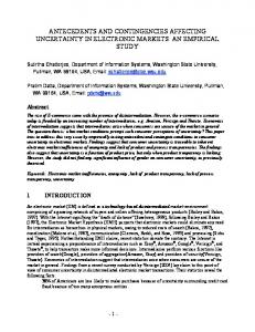
with corr(dwS , dwV ) = ρ. This model allows for volatility clustering through the autoregressive component of volatility, and for a leverage effect through a negative correlation coefficient ρ, which translates into negative skewness of the return distribution.14 Note also that the AF-SV model √ implies that the instantaneous change in variance is heteroskedastic via the V term in the volatility diffusion. In order to explore the AF-SV model further consider the instantaneous volatility dynamic implied by the model. Using Ito’s lemma, we can write √ 1 (3) d V = μ(V )dt + σdwV 2 Note that the the AF-SV model implies that the instantaneous change in volatility should be √ Gaussian and homoskedastic: V does not show up in any way in the diffusion term for d V . This implication is strong and can be assessed empirically quite easily. Using daily realized volatilities from 1990 to 2002, the top panel of Figure 1 shows a quantilequantile (QQ) plot of the daily realized volatility changes compared with the Gaussian distribution.15 The deviation of the data points from the straight line indicate that the Gaussian distribution is not a good assumption for daily changes in volatility. The observed tails (both left 13 14

See for example Andersen, Bollerslev, Diebold and Labys (2003), and Ait-Sahalia, Mykland and Zhang (2005). Note that following Chernov and Ghysels (2000), Eraker, Johannes and Polson (2003) and Eraker (2004) we use

a simple constant specification for the stock return drift. 15 The realized volatility data was graciously provided to us by and is documented in Andersen, Bollerslev and Diebold (2005).

6

and right) are considerably fatter than the normal distribution would suggest. The middle panel in Figure 1 scatter plots the daily volatility changes against the daily volatility level. According to the AF-SV model this scatter plot should reveal no systematic patterns. However, as the volatility level increases on the horizontal axis a cone-shaped pattern in the daily volatility changes on the vertical axis is apparent. Confirming this pattern, the bottom panel of Figure 1 scatter plots the absolute daily volatility changes against the daily volatility level. A simple OLS regression line is shown for reference. Notice a clearly positive relationship between the volatility level and the magnitude of volatility changes. This pattern is in conflict with the homoskedastic volatility implication of the AF-SV model. In the implementation below we will rely on the dynamics for log variance which using Ito’s lemma can be written as

1 d ln(V ) = μ(V )dt + σ √ dwV (4) V Notice that the log variance dynamics also imply heteroskedastic instantaneous changes and this time with a factor of

2.2

√1 V

.

The Non-Affine Stochastic Volatility Model (NA-SV)

When departing from the affine model framework many directions can be taken. We focus on a process which has the same number of parameters as the affine SV model above and which has appealing empirical implications as we shall see shortly. We will assume the following NA-SV dynamic dS = μSdt + dV

√ V SdwS

= κ(θ − V )dt + σV dwV

(5) (6)

with corr(dwS , dwV ) = ρ. In this model the innovations are scaled by the conditional variance rather than by the square root of the conditional variance as is the case in the AF-SV model. To explore this model further, consider now the implications of this model for instantaneous volatility dynamics. We can write √ 1 √ d V = μ(V )dt + σ V dwV 2

(7)

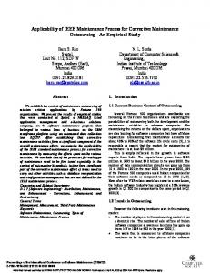
so that volatility changes are heteroskedastic as Figure 1 suggests they should be. Note next that the NA-SV model implies that the instantaneous changes in log variance are homoskedastic. Using Ito’s lemma we can write d ln(V ) = μ(V )dt + σdwV Figure 2 summarizes the empirics of realized log variances. The top panel shows that daily changes in the realized log variances follow the Gaussian distribution quite closely. This feature is 7

implied by the NA-SV model and it clearly differs from the finding for the daily volatility changes in Figure 1. Furthermore, the middle panel of Figure 2 shows the scatter of daily log variance changes against the log variance level. Note that no cone-shaped pattern is apparent. The bottom panel in Figure 2 confirms this first impression and shows a virtually flat line when regressing absolute changes in log variance on log variance levels. Note that the absence of a clear relationship between changes in the log variances and the log variance level in Figure 2 lends credence to the NA-SV specification but it also casts further doubt on the AF-SV specification where the instantaneous changes in log variance are heteroskedastic as shown in (4) above.

2.3

The Affine GARCH Model (AF-GARCH)

Heston and Nandi (2000) propose a class of affine GARCH models (AF-GARCH) that allow for a closed-form solution for the price of a European call option. We investigate the GARCH(1,1) version of this model, which is given by p ln(St+1 ) = ln(St ) + r + pVt + Vt zt+1 ´2 ³ p Vt = w + bVt−1 + a zt − c Vt−1

(8) (9)

where St+1 denotes the underlying asset price, r the risk free rate, p the price of risk and Vt the daily variance for day t + 1 which is known at the end of day t.16 The zt+1 shock is assumed to be i.i.d. N (0, 1). The Heston-Nandi model captures time variation in the conditional variance in ways similar to Engle (1982) and Bollerslev (1986). The parameter c represents the leverage effect, which captures the negative relationship between returns and volatility (Black (1976)) and results in a negatively skewed conditional distribution of multi-day returns. In order to explore the model further, notice that variance persistence can be computed via b + ac2 ≡ 1 − κ and the unconditional variance can be computed via ¡ ¢ (w + a)/ 1 − b − ac2 = (w + a)/κ ≡ θ

Now we can rewrite the variance process as

Vt − Vt−1 = κ(θ − Vt−1 ) + avt ¡¡ 2 ¢ ¢ √ where vt = zt − 1 − 2czt Vt−1 , and where we have p StdDevt−1 (vt ) = 2 + 4c2 Vt−1

(10)

(11)

The fact that the variance appears in a square-root form in (11) suggests the AF-GARCH model’s relationship with the AF-SV model considered above. 16

The timing convention we use here is slightly non-standard in the GARCH literature but it facilitates comparisons

with the SV models.

8

2.4

The Non-Affine GARCH Model (NA-GARCH)

We compare the AF-GARCH model with the non-affine NGARCH model of Engle and Ng (1993). We choose the NGARCH model because it is relatively easy to analyze, and because it has been shown to provide a good description of underlying equity returns.17 We will refer to this model as NA-GARCH. The model is given by p p ln(St+1 ) = ln(St ) + r + p Vt − 0.5Vt + Vt zt+1 Vt = w + bVt−1 + aVt−1 (zt − c)2

(12) (13)

As in the AF-GARCH model, we can define the variance persistence via ¢ ¡ b + a 1 + c2 ≡ 1 − κ

and the unconditional variance can be computed via

¢¢ ¡ ¡ w/ 1 − b − a 1 + c2 = w/κ ≡ θ

Now we can rewrite the variance process as

Vt − Vt−1 = κ(θ − Vt−1 ) + aVt−1

¡¡ 2 ¢ ¢ zt − 1 − 2czt

(14)

Notice that the variance of the shock term is 2 + 4c2 so that we have Vt − Vt−1 = κ(θ − Vt−1 ) + σVt−1 vt

√ ¡¡ ¢ ¢ √ where σ = a 2 + 4c2 and vt = zt2 − 1 − 2czt / 2 + 4c2 . Notice also that we have −2c ≡ρ Corr (zt , vt ) = √ 2 + 4c2

all of which suggests the NA-GARCH model’s close relationship with the NA-SV model. Note that this model differs in some subtle ways from the Heston-Nandi model in (8)-(9). The Heston-Nandi model was engineered with the specific purpose of yielding closed-from option prices. The specification in (12)-(13) does not yield closed form option prices, but was designed to provide a good fit to the underlying equity returns. The question of interest is if the restrictions built into affine models such as (8)-(9) reduce the ability of the model to fit the options data. 17

See for example Duan (1997).

9

3

Volatility Model Implementation

The Heston AF-SV model has been investigated empirically in a large number of studies. Often it is used as a building block together with models of jumps in return and volatility.

For our

purpose, it is important to note that the model can be estimated and investigated empirically using a number of different techniques. First, the model’s parameters can be estimated using a single cross-section of option prices (for example see Bakshi, Cao and Chen (1997)). A second type of implementation of the Heston model uses multiple cross sections of option prices but does not use the information in the underlying asset returns. Instead, for every cross section a different initial volatility is estimated, leading to a highly parameterized problem (see for instance Bates (2000) and Huang and Wu (2004)). A third group of papers provide a likelihood-based analysis of the stochastic volatility model. See for example Ait-Sahalia and Kimmel (2005), Bates (2004), Jones (2003), and Eraker (2004), who provides a Markov Chain Monte Carlo analysis. Finally, Chernov and Ghysels (2000) use the efficient method of moments and Pan (2002) uses a method of moments technique as well. These methods can also combine information in the options data as well as the underlying returns. In this paper we implement the SV models in a novel way. This is mainly motivated by our desire to compare the performance of discrete-time and continuous-time methods in a meaningful way. For all the four models our implementation uses the nonlinear least squares (NLS) estimation techniques to minimize $M SE =

1 X (Ci,t − Ci (Vt ))2 NT

(15)

t,i

with respect to the structural parameters.

NT =

T P

Nt , T denotes the total number of days

t=1

included in the options sample, Nt is the number of options with various strikes prices and maturities included in the sample at date t, Ci,t is the market price of option i quoted on day t and Ci (Vt ) is the model price. In our opinion, matching the objection function used in parameter estimation with the function subsequently used to evaluate the models ensures the best possible performance of the models in- and out-of-sample. This is motivated by the insights of Granger (1969), and Weiss and Andersen (1984) who demonstrate that the choice of objective function (also labeled loss function) is an integral part of model specification. It follows that estimating a model using one objective function and evaluating it using another one amounts to a suboptimal choice of objective function. Christoffersen and Jacobs (2004b) demonstrate that this issue is empirically relevant for the estimation of the deterministic volatility functions in Dumas, Fleming and Whaley (1998). We implement the SV models in a way that is consistent with these insights.

10

3.1

The AF-SV Model

The problem with (15) is that the spot volatility Vt is an unobserved latent factor in the two SV models. Rather than treating the spot volatility on each day as extra parameters to be estimated, we will apply a filtering technique on observed index returns in order to avoid overfitting. Filtering volatility on returns also ensures that the option valuation model is consistent with both options and returns data. Our implementation uses the Auxiliary Particle Filter (APF) algorithm for the two SV models.18 As shown by Pitt and Shephard (1999) the APF offers a convenient filtering algorithm for non-linear models such as the stochastic volatility model we consider here. Because the APF procedure is relatively new in finance, we now discuss the implementation of this method in more detail.19 3.1.1

Volatility Transformation and Discretization

To prevent V from becoming negative, we work with f (V ) = ln(V ). We also work with the log stock returns. Using Ito’s lemma, the dynamic of interest is therefore ¶ µ √ 1 d ln(S) = μ − V dt + V dwS 2 µ ¶ 1 1 1 κ(θ − V ) − σ 2 dt + σ √ dwV d ln(V ) = V 2 V

(16)

Note that the equations in (16) specify how the unobserved state is linked to observed stock prices. This relationship allows us to infer the volatility path using the returns data. We first need to discretize (16). There are different discretization methods and every scheme has certain advantages and drawbacks. We use the Euler scheme which is easy to implement and has been found to work well for this type of applications.20 Discretizing (16) gives ¶ p µ 1 ln(St+1 ) = ln(St ) + μ − Vt + Vt εSt+1 2 µ ¶ 1 1 2 1 ln(Vt+1 ) = ln(Vt ) + κ (θ − Vt ) − σ + σ √ εVt+1 Vt 2 Vt

(17) (18)

We implement the discretized model in (17) and (18) using daily returns, and all parameters except the unconditional variance, θ, will be expressed in daily units below. The model is characterized by six structural parameters: μ, κ, θ, σ, λ and ρ for which we have to choose a set of starting values. 18

We have also implemented the Sampling-Importance-Resampling (SIR) particle filter as a robustness check, and

this yields similar results. 19 Johannes, Polson and Stroud (2002) discuss the use of the particle filter to estimate parameters for continuoustime jump-diffusion models on returns data. 20 See for example Eraker (2001).

11

Subsequently, we have to choose an initial variance V0 (the starting value for the variance path). We set the initial variance equal to the model-implied unconditional variance, V0 = θ.21 Our optimization algorithm minimizes (15) using an iterative procedure on the structural parameters. At each iteration, the volatility is filtered using the information embedded in observed returns and the structural parameters. Using the filtered volatility and the structural parameters, option prices are computed according to Heston’s formula and the M SE is calculated. This procedure searches in the structural parameter space until the optimum is reached. We now describe the volatility filtering step. 3.1.2

Filtering the volatility path using the APF algorithm

The Auxiliary Particle Filter (APF) algorithm relies on the approximation of the true density of the state Vt+1 by a set of N discrete points or particles that are updated iteratively through equations oN n j j , Wt+1 of (17) and (18). The filter is implemented by deriving the empirical distribution Vt+1 j=1 oN n Vt+1 , conditional on knowledge of the empirical distribution Vtj , Wtj of Vt . This implemenj=1

tation proceeds in three steps. First, among the set of particles describing the distribution of Vt ,

we select the high probability particles. Second, we propagate these selected (resampled) particles forward. Third, we assign weights to each new particle and get the discrete empirical distribution of Vt+1 . At the end of Step 3, we obtain a set of N particles describing the density of Vt+1 . The details of the three steps are given in the appendix. Steps 1, 2 and 3 are repeated for t = 1, ...T . To obtain the filtered volatility path, we then compute V¯t+1 =

N X j j Wt+1 Vt+1

(19)

j=1

for each t. 3.1.3

Computing option prices and evaluating the loss function

In order to price options with the AF-SV model we need the risk neutral dynamics. Under the assumption that the volatility risk premium λ(S, V, t) is equal to λV , the risk neutral dynamic expressed in terms of the physical parameters and λ is √ dS = rSdt + V Sdw∗S dV

21

√ = (κ(θ − V ) − λV ) dt + σ V dw∗V √ = (κ + λ)(κθ/(κ + λ) − V )dt + σ V dw∗V

(20) (21)

In order to mitigate the impact of the choice of the initial variance V0 we start iterating on the volatility dynamic

on the day corresponding to four years before the first observed option price. This initial date is held fixed in all the estimation samples and for all the models.

12

with corr(dw∗S , dw∗V ) = ρ. Heston (1993) demonstrates that this model admits a closed form solution for option prices, which can be written as C(Vt ) = SP1 − Ke−r(T −t) P2

(22)

where the equations for P1 and P2 are given in the appendix. ¡ ¢ We are now in a position to evaluate option prices Ci V¯t based on the filtered volatility path and using Heston’s closed form solution in equation (22). We subsequently evaluate the loss function ¡ ¢ (15), using Ci V¯t for the model price Ci (Vt ). We use a standard numerical optimization routine

to update the model parameters and iterate until convergence is achieved.

Notice that the methodology we have suggested here for estimating the continuous time stochastic volatility model relies on the same information set and uses the same objective function as the two discrete time models, which will be discussed in detail below. This will allow for a fair empirical comparison between models.

3.2

The NA-SV Model

In order to compute option prices under the NA-SV dynamics we assume that the volatility risk premium λ(S, V, t) is equal to λV , so that the risk neutral dynamic expressed in terms of the physical parameters and λ is √ V Sdw∗S

(23)

= (κ(θ − V ) − λV ) dt + σV dw∗V

(24)

dS = rSdt + dV

= (κ + λ)(κθ/(κ + λ) − V )dt + σV dw∗V

with corr(dw∗S , dw∗V ) = ρ. Note that the assumption on the volatility risk premium is the same as in the AF-SV model. In both cases the risk-neutralization can be obtained using a no-arbitrage argument, but in the AF-SV case the risk-neutral dynamic can also be obtained using a utility-based argument.

In order to

isolate the importance of the volatility dynamic, we keep the volatility risk premium specifications constant across the affine and non-affine SV models.22

While clearly empirically appealing, the

NA-SV model presented here has an unobserved variance factor and no closed form option valuation formula. Thus we need to implement it using the auxiliary particle filter to construct the variance path (as in AF-SV) and Monte Carlo simulation to calculate the option prices. We use 1,000 simulated paths and a number of numerical techniques to increase numerical efficiency: the empirical martingale method of Duan and Simonato (1998), stratified random numbers, antithetic variates and a control variate technique. The model is estimated by minimizing (15) with respect to the structural parameters μ, κ, θ, ρ, σ, and λ. 22

See Lewis (2000) for a thorough discussion of these issues.

13

3.3

The AF-GARCH Model

The risk-neutral dynamics for the GARCH(1,1) model (8)-(9) are given by23 p ∗ ln(St+1 ) = ln(St ) + r − 12 Vt + Vt zt+1 p Vt = w + bVt−1 + a(zt∗ − (c + p + 0.5) Vt−1 )2

(25)

∗ with zt+1 ∼ N (0, 1) under the risk neutral measure. At time t, a European call option with strike

price K that expires at time T can be calculated from

C (Vt ) = St P1 − Ke−r(T −t) P2 where the formulas for P1 and P2 are provided in the appendix. We provide an analysis of this model using data on equity option prices as well as the time series of underlying equity returns. In order to value options at each date t, we need an estimate of the conditional volatility Vt on that particular date. One of the appealing aspects of discrete-time GARCH models is that this filtering problem is extremely simple. Indeed, the filtering problem is solved by noting that from (8) we have p zt+1 = (Rt+1 − r − pVt ) / Vt

(26)

where Rt = ln(St /St−1 ). Substituting (26) in (9), it can be seen that the updating from Vt−1 to Vt is done exclusively using observables p p Vt = w + bVt−1 + a((Rt − r) / Vt−1 − (c + p) Vt−1 )2

(27)

Model parameters are again obtained by using the nonlinear least squares (NLS) estimation techniques to minimize (15). The implementation is therefore relatively simple: the NLS routine is called with a set of parameter starting values. The variance dynamic in (27) is then used to update the variance from day to day and the GARCH(1,1) option valuation formula from Heston and Nandi (2000) is used to compute the model prices.

3.4

The NA-GARCH Model

The risk-neutral dynamics required for option valuation with the NA-GARCH model (12)-(13) can be obtained as ln(St+1 ) = ln(St ) + r − 0.5Vt +

p ∗ Vt zt+1

(28)

Vt = w + bVt−1 + aVt−1 (zt∗ − (c + p))2

23

For the underlying theory on risk neutral distributions in discrete time option valuation see Rubinstein (1976),

Brennan (1979), Amin and Ng (1993), Duan (1995), Camara (2003), Heston and Nandi (2000) and Schroder (2004).

14

∗ with zt+1 ∼ N (0, 1). As in the case of the NA-SV model, no closed-form solution exists for option

valuation in the NA-GARCH model. Instead, Monte Carlo simulation is required. We can estimate the model by minimizing (15), using the updating rule ³h i ´2 p Vt = w + bVt−1 + aVt−1 (Rt − r + 0.5Vt−1 ) / Vt−1 − (c + p)

(29)

Option prices are computed numerically according to

C (Vt ) = e−r(T −t) Et∗ [M ax(ST − K, 0)] where the expectation is calculated by Monte Carlo simulation of the daily returns from (28). We use the same Monte-Carlo setup as in the NA-SV case, with 1,000 simulated paths and using the empirical martingale method of Duan and Simonato (1998), stratified random numbers, antithetic variates and a control variate technique.

4

Empirical Results

This section presents the empirical results.

We first discuss the data, followed by an empirical

evaluation of the four models under investigation and a detailed discussion of the differences in performance of these models in- and out-of-sample.

4.1

Data

We conduct our empirical analysis using three years of data on S&P 500 call options, for the period 1993-1995. We apply standard filters to the data following Bakshi, Cao and Chen (1997). We only use Wednesday and Thursday options data. For the in-sample analysis, we use the Wednesday data. Wednesday is the day of the week least likely to be a holiday. It is also less likely than other days such as Monday and Friday to be affected by day-of-the-week effects. The decision to pick one day every week is to some extent motivated by computational constraints. The optimization problems are fairly time-intensive, and limiting the number of options reduces the computational burden. Using only Wednesday data allows us to study a fairly long time-series, which is useful considering the highly persistent volatility processes. An additional motivation for only using Wednesday data is that following the work of Dumas, Fleming and Whaley (1998), several studies have used this setup.24 We obtain three sets of parameter estimates in the in-sample analysis. We simply split the three years of data in three datasets, one for each calendar year, and perform annual estimation exercises. For each estimation sample, we apply the volatility updating rules using returns and starting from the model implied unconditional variance on January 2, 1989. 24

See for instance Heston and Nandi (2000).

15

Table 1 presents descriptive statistics for the options data for the 1993-1995 Wednesday insample data by moneyness and maturity. Panels A and B indicate that the dataset contains a rich selection of options across moneyness and maturity. Panel C displays the volatility smirk in the data. The slope of the smirk clearly differs across maturities. We summarize the data for all three estimation samples in one set of tables to save space. Descriptive statistics for the yearly samples (not reported here) reveal similar stylized facts. The slope of the smirk changes over time, but the smirk is present throughout the sample. The top panel of Figure 3 gives some indication of the pattern of implied volatility over time. For the 156 Wednesdays of options data used in the empirical analysis, we present the average implied volatility of the options on each Wednesday. It is evident from Figure 3 that there is substantial clustering in implied volatilities. The bottom panel of Figure 3 presents a time series for the 30-day at-the-money volatility (VIX) index from the CBOE for our sample period. A comparison with the top panel clearly indicates that the options data in our sample are representative of market conditions, although the time series based on our sample is of course a bit more noisy due to the presence of options with different moneyness and maturities. After conducting three in-sample estimations, we proceed to conducting separate out-of-sample analyses for each of the three sample years using the trading day following each in-sample Wednesday. We refer to these datasets as the Thursday data. Table 2 presents descriptive statistics for the out-of-sample Thursday data.

The patterns in the data are clearly similar to those in the

in-sample data in Table 1. Note that we are deliberately working with a relatively tranquil time-period for option prices. We are estimating four models that are simple in terms of their volatility memory properties (single factor models) and simple in terms of shock innovations (Gaussian), but which vary in their specifications of how shocks to volatility change the level of volatility. Increasing the sample period length to including more interesting episodes such as the 1990-91 recession or the 1998 LTCM crisis would be useful but would require more sophisticated models potentially including multiple volatility components and non-Gaussian innovations. We leave such analysis for future work.

4.2

Parameter Estimates and Option Mean-Squared-Errors

Table 3 presents the parameter estimates for each of the four models and for each of the three annual estimation samples. All parameters are reported in daily units except for the unconditional variance θ which we report in annual standard deviations. The parameters for the SV models are directly interpretable individually; for example, κ denotes the daily variance mean reversion. The most striking aspect of the estimates is that the correlation parameter ρ hits the prespecified boundary of -0.999 for the NA-SV model in 1993 and 1994 and gets very close to it in 1995. The correlation in the AF-SV model is also large in magnitude in every year.

16

These estimates, which are driven by the objective to minimize the option price squared errors, indicate that the option prices drive the correlations to be much larger in magnitude than the estimates typically found in papers estimating the models on returns only. Below we will estimate the four models on returns only, which yields correlation estimates that are indeed very close to those reported in the literature. We readily acknowledge that the parameter estimates indicate potential misspecification of the model and that further work on the models is needed.

The

objective of this paper is not to find the best possible affine or non-affine model. We merely want to demonstrate that a simple (and possibly misspecified) non-affine model improves significantly on the benchmark affine model. For the AF-GARCH and NA-GARCH models, we report the parameters from the specifications in (10) and (14) in order to facilitate comparison with the SV models. For the non-affine models the parameters are quite comparable across models. For the affine models, a comparison is less straightforward, partly because the conditional correlation is time-varying in the AF-GARCH model as we will discuss further below. To further facilitate the comparison between the different models, the last two columns in Table 3 report the risk neutral variance mean-reversion and unconditional volatility. The variance meanreversion is close to zero for all models, which is consistent with other findings in the literature. Due to the negative price of volatility risk in the SV models and the positive price of equity risk in the GARCH models, the risk neutral mean-reversion is lower than the physical mean-reversion in all models. For the same reason, the unconditional volatility is larger under the risk-neutral measures. Mean-reversion is always smallest in the AF-SV specification. The physical unconditional volatility displays some variation over time, but the risk-neutral unconditional volatility is actually quite stable. Figure 4 provides further perspective on the similarities and differences between the four models by reporting volatility sample paths for the models. The figure plots volatility paths for 1993-1995 from the four models using the three sets of parameters estimates from 1993, 1994, and 1995 respectively. It can be seen that the sample paths show some similarities across models and across estimates. However, it does appear that volatility itself is less volatile in the AF-SV model than in the other three models. We will investigate this issue further below. The in- and out-of-sample RMSEs from the four models are reported in Table 4 for each of the three samples. First note that the NA-SV model is best overall and the AF-SV model is worst overall both in- and out-of-sample. The overall difference between these models is 25.5% in-sample and 27.5% out-of-sample. The performance of the NA-GARCH and NA-SV models is similar in- and out-of-sample with the NA-SV model performing somewhat better overall. This correspondence between the fit of the non-affine continuous-time and discrete-time models does not hold for the affine models. The fit of the AF-GARCH model falls in between the AF-SV and the

17

non-affine models. The AF-GARCH is approximately 10.2% better than the AF-SV in-sample and approximately 7.6% better out-of-sample. Looking across the three samples, a robust conclusion obtains: the non-affine models substantially outperform the affine models in every year, both inand out-of-sample. Table 5 tests the significance of the difference in weekly RMSE. In order to circumvent having to specify the variance matrix of the options errors which are likely to have strong maturity, moneyness and dynamic dependencies we simply test the difference in the average weekly RMSE across models. When doing so we use the Diebold and Mariano (1995) test allowing for autocorrelation in the weekly RMSEs. The Diebold-Mariano test has an asymptotic normal distribution and the results in Table 5 show that when the AF-SV model is taken as a benchmark, the two non-affine models are significantly better in-and out-of-sample, and the AF-GARCH model is significantly better insample. When the NA-SV model is used as a benchmark the two affine models are significantly worse, but the NA-GARCH model is not significantly different from the NA-SV. We thus conclude that the differences between affine and non-affine models are significant but the difference between the NA-GARCH and NA-SV models is not significant at conventional levels. We now analyze the dynamic performance of the four models in more detail. Figures 5 and 6 address the performance of the models over time. The four panels in Figure 5 present the in-sample RMSE on a week-by-week basis for each of the four models. It can clearly be seen that the four models display important similarities in terms of the dynamic pricing errors, however, the AF-SV model appears to be somewhat different from the other three models. Notice in particular the larger weekly RMSE in the first half of 1994 which corresponds to the period when the VIX in Figure 3 was high. This observation is confirmed by inspecting the week-by-week in-sample bias in Figure 6 where the AF-SV model underprices options around the peak of the VIX. Notice also how in 1995 the AF-SV model consistently overprices the options in almost every week of the year. This is less so in the other three models.

4.3

Pricing Errors Across Moneyness and Maturity

Tables 6 and 7 present an analysis of the in- and out-of-sample RMSE by moneyness and maturity. The most important conclusion from Tables 6 and 7 is that the two non-affine models outperform the corresponding affine models for almost every cell in the moneyness-maturity matrix, in-sample as well as out-of-sample. Consider in particular the All moneyness rows and the All maturities columns in each panel of Tables 6 and 7. It is striking that the NA-SV model performs the best in virtually every single case and the NA-GARCH model performs second best also in virtually every single case. These tables also allow for some other important conclusions. For example, consider the difference between the AF-SV and AF-GARCH models. While the overall RMSE difference between

18

the two models in Table 5 is approximately 8-10% in- and out-of-sample, there are important variations in the relative performance of the models across maturity. The overall RMSE of the AF-SV model is larger than that of the AF-GARCH model, but for short-maturity options the AF-SV model actually performs better. While perhaps somewhat surprising, this finding could be due to the fact that our mean-squared pricing error objective function puts relatively little weight on the inexpensive short-term options. Tables 8 and 9 report the in- and out-of-sample bias across moneyness and maturity. In these tables we are looking for systematic over or underpricing of options with particular moneyness and maturity characteristics. Consider for example the AF-SV model in Panel A of Table 8. It has an overall bias of 24 cents, but more importantly it systematically overprices out-of-the-money calls and underprices in-the-money calls. Such systematic biases are much less apparent for the other three models in Table 8. Table 9 shows the same pattern as Table 8 for the AF-SV model, but it also shows this pattern for the NA-GARCH model. Figures 7.A-C provide additional intuition for the differences in the cross-sectional performance between the four models.

Using each of the three sets of estimates, these figures depict the

simulated state price densities for a one-month, three-month and one-year horizon. Each row of panels reports the risk neutral distribution of the standardized index return according to the AF-SV, NA-SV, AF-GARCH and NA-GARCH models respectively. The normal distribution corresponding to the Black-Scholes model is shown in dots for reference. The left column reports the 1-month horizon, the center column the 3-month horizon distribution and the right column shows the 1-year distribution. The distributions are constructed by simulating daily returns from each model setting the initial spot variance equal to the unconditional variance. Kernel density estimates are then constructed from the standardized simulated returns. It can clearly be seen that deviations from normality are large, and that the estimated parameters for the four models imply different deviations from normality. It is interesting to note that the leverage effects generate a substantial amount of skewness in the risk-neutral return distributions, particularly in the NA-SV model, even at the 1-year horizon. This finding is consistent with the nonparametric evidence in Ait-Sahalia and Lo (1998) that skewness persists at long horizons. It is also consistent with the biases found in Table 8 and 9: Only the NA-SV model consistently provides enough skewness in the state-price density to avoid systematically overpricing the out-of-the-money calls and underpricing the in-the-money calls.

4.4

Conditional Moment Dynamics

While the state price densities shown in Figures 7.A-C illustrate the properties of the option pricing models when fixing the conditional volatility at its unconditional level, ultimately, the option prices from the different models are determined by the dynamics of the conditional density. Therefore,

19

we now discuss model differences by focusing on various conditional moments of the return density. In order to asses the different models’ ability to generate time-variation in the asymmetry of the return distribution, Figure 8 plots the conditional covariance between returns and variances for each model. We refer to this conditional covariance as the conditional leverage path, which for the four models is given by AF-SV :

covt (Rt+1 , Vt+1 ) = σρVt

NA-SV :

covt (Rt+1 , Vt+1 ) = σρVt

3/2

AF-GARCH :

covt (Rt+1 , Vt+1 ) = −2acVt

NA-GARCH :

covt (Rt+1 , Vt+1 ) = σρVt

3/2

(30)

Notice that critical differences between the affine and non-affine models show up very prominently in these conditional moments. The power on the variance differs between the affine and the non-affine models. For each model we plot in Figure 8 the daily conditional leverage path during 1993-1995, annualized by multiplying by 252. The left column uses the 1993 estimates from Table 3, the middle column uses 1994 estimates, and the right column uses the 1995 estimates. The four rows of panels correspond to the AF-SV, NA-SV, AF-GARCH and NA-GARCH models respectively. The main conclusion is that for all three sets of estimates the non-affine models imply more variation over time in the leverage effect. Notice that particularly the AF-SV model is very different from the other three models. Given the importance of the leverage effect for option valuation, this may be a very important factor in explaining the differences in the fit between affine and non-affine models documented in Tables 4 and 5. Option prices are a function of the conditional variance, and therefore the variation in option prices over time is related to the conditional variance of variance. The conditional variance of variance of returns for the four models is given by AF-SV :

V art (Vt+1 ) = σ 2 Vt

NA-SV :

V art (Vt+1 ) = σ 2 Vt2

AF-GARCH :

V art (Vt+1 ) = 2a2 + 4a2 c2 Vt

NA-GARCH :

V art (Vt+1 ) = σ 2 Vt2

(31)

Notice again that the power on Vt in these conditional moments indicate important differences between affine and non-affine models. The conditional variance shows up in levels in the affine models and in squared form in the non-affine models.25 Figure 9 reports the empirical results for 25

Notice also that in the affine GARCH model the variance of variance will be constant when c = 0 whereas this

is not the case in the non-affine models nor in the AF-SV model.

20

the volatility of variance. For each model, we plot the daily conditional volatility of variance path during 1993-1995 annualized by multiplying by 252. The left column uses the 1993 estimates from Table 3, the middle column uses 1994 estimates, and the right column uses the 1995 estimates. The four rows of panels correspond to the AF-SV, NA-SV, AF-GARCH and NA-GARCH models respectively. Figure 9 indicates that for all sets of estimates the non-affine models display much more time-variation in the volatility of variance. This is particularly true versus the AF-SV model and it is particularly true during the first half of 1994 when the level of volatility peaks (see Figure 3). These differences between the models further help us understand the superior fit of the non-affine models.

4.5

Comparing the SV and GARCH Results

The main objective of the empirical comparison between the four option valuation models is to investigate the implications of assuming an affine model structure. While this is a simple and important question, the available literature does not contain a conclusive answer, although specification tests in Jones (2003) indicate that generalizations of the affine framework might be useful. Our use of the Auxiliary Particle Filter, which is new in the option valuation literature, allows us to compare the benchmark AF-SV Heston (1993) model with a simple NA-SV model along a dimension such as the dollar RMSE. Our results are very clear: while the affine SV model is analytically convenient, it substantially underperforms the non-affine SV model. Interestingly, the discrete-time NA-GARCH model also outperforms the AF-GARCH model, but the differences in fit are much smaller. These empirical results also allow us to comment on the relationship between the empirical performance of discrete-time and continuous-time models. Existing theoretical limit results have sometimes been interpreted as suggesting that the performance of these models ought to be similar, and indeed as suggesting that a study of the empirical differences is not worthwhile. However, this interpretation is contradicted at a theoretical level by the fact that a single discrete-time model can be linked with several continuous-time limits and vice versa. Our empirical results clearly confirm that the relationship between discrete-time and continuous-time models is far from obvious. Our most important result in this respect is that the AF-SV Heston (1993) model, which is one of the most popular option valuation models, performs rather poorly when compared to the AF-GARCH Heston-Nandi (2000) model. This may seem surprising, because Heston and Nandi (2000) demonstrate that a restricted version of the Heston (1993) model can be obtained as a limit of their model. However, close inspection of the proof in Heston and Nandi (2000) reveals that this limit result is a special case, and the restricted Heston (1993) limit may not be the limit that is most relevant from an empirical perspective. In order to explore this issue further, consider the conditional correlation between returns and

21

volatility for the four models, which can be computed from (30) and (31) AF-SV :

σρVt =ρ Corrt (Rt+1 , Vt+1 ) = √ Vt σ 2 Vt 3/2

NA-SV : AF-GARCH :

σρV Corrt (Rt+1 , Vt+1 ) = p t =ρ Vt σ 2 Vt2 −2cVt Corrt (Rt+1 , Vt+1 ) = p (2 + 4c2 Vt )Vt 3/2

NA-GARCH :

σρV Corrt (Rt+1 , Vt+1 ) = p t =ρ Vt σ 2 Vt2

(32)

Clearly an important difference is that for the AF-GARCH model the conditional correlation is time-varying whereas it is constant for the other three models. Thus, while the AF-GARCH and AF-SV models are similar in many ways, they differ along this important dimension. Figure 10 plots the time-varying correlation in the AF-GARCH during the period 1993-1995 for the three sets of estimates obtained in Table 3. The horizontal line in each panel shows the estimated constant correlation in the AF-SV model for the relevant year. Notice that the time-varying correlation in the AF-GARCH model typically varies substantially from the constant correlation in the AFSV model. This added flexibility in the AF-GARCH model can potentially explain some of the improvement in option RMSE over the AF-SV model.

4.6

Estimation on Returns Only

The estimates in Table 3 where intentionally obtained by minimizing the object of interest, which in this paper was taken to be the option price mean squared error. The advantage of the estimation methodology we have suggested is that it can be tailored to any objective function of interest. Instead of option price MSE, the objective of interest could be relative price MSE or implied volatility MSE. More economically based objectives such as hedging error variance or trading profits could be entertained as well. Consider the special case where the researcher is interested not in option price fitting but instead in a return—based likelihood objective.26 In the two discrete time GARCH models the optimization problem is straightforward as the log-likelihood is simply given by T

ln(L) = −

¢ 1 X¡ ln(2π) + ln (Vt ) + zt2 /Vt 2 t=2

where zt is obtained from the relevant return equation and Vt from the variance dynamics. The initial observation can be used as a starting condition setting V1 to θ. Using the discretization in equations (17) and (18) and using the auxiliary particle filter we can similarly estimate the two SV models on returns by maximizing the function analog to the 26

See also Ait-Sahalia and Kimmel (2005).

22

log-likelihood T

ln(L) = −

¡ ¢ ¢ 1 X¡ ln(2π) + ln V¯t + zt2 /V¯t 2 t=1

where V¯t is now computed from the particle filter as in equation (19).

Table 10 shows the results from this estimation exercise using daily returns on the S&P500 from January 1, 1980 to December 31, 1999. Note that the objective function is much larger for the NASV than the AF-SV and similarly the NA-GARCH objective is much larger than the AF-GARCH objective. Thus, returns also favor the non-affine specifications in both the SV and the GARCH case.

Notice also that the ρ and c parameters which capture the shock correlations in the four

models are much smaller in magnitude in Table 10 than those reported in Table 3. The estimates in Table 10 are very close to the return-driven estimates found for example in Eraker, Johannes and Polson (2003) who also use the 1980-1999 sample period.

5

Conclusions and Directions for Future Work

This paper has provided an empirical comparison of affine and non-affine option valuation models. The in-sample RMSE of a non-affine stochastic volatility model (NA-SV) is approximately 25.5% lower than that of the affine Heston (1993) model (AF-SV), and the out-of-sample RMSE is approximately 27.5% lower. The non-affine model outperforms the affine model in all three in-sample exercises as well as in all three out-of-sample exercises. The non-affine model also outperforms the affine model for virtually all moneyness and maturity categories. We also study the differences between the affine discrete-time GARCH option model of Heston and Nandi (2000) (AF-GARCH) and a non-affine GARCH model (NA-GARCH). Interestingly, the differences in RMSE between these two models are smaller, approximately 10% in-sample and 15% out-of-sample.

While the performance of the NA-GARCH model is very similar to that of

the NA-SV model, the AF-GARCH model performs significantly better than the AF-SV model, in-sample as well as out-of-sample. The AF-GARCH does not lead to a uniformly better fit than the AF-SV model: The AF-SV model outperforms the AF-GARCH model for short maturities. These empirical results allow us to draw two conclusions. First, regarding the distinction between affine and non-affine models: while the focus of the option valuation literature on affine models is well motivated, because the resulting closed-form solutions are extremely convenient, our results suggest that this analytical convenience comes at a price, and non-affine models need to be studied more extensively. Second, our results are relevant for the relationship between continuoustime and discrete-time option valuation models. Our empirical results on this issue have to be interpreted cautiously and do not allow for general conclusions. In our opinion, the most important aspect of our empirical comparison between the empirical performance of discrete-time and

23

continuous-time models is what it says about the performance of some important benchmarks in the literature. Our most interesting conclusion in this respect is that the most important model in the literature on option valuation under stochastic volatility, the AF-SV Heston (1993) model, performs rather poorly when compared to the AF-GARCH model in Heston and Nandi (2000).

This may seem

surprising, because Heston and Nandi (2000) demonstrate that a restricted version of the Heston (1993) model can be obtained as a limit of their model. However, close inspection of the proof in Heston and Nandi (2000) reveals that this limit result is a very special case, and the restricted Heston (1993) limit may not be the limit that is most relevant from an empirical perspective. Note also that the AF-SV Heston (1993) model is effectively a model with two stochastic shocks, while the AF-GARCH Heston and Nandi (2000) model, like other GARCH models, only contains one stochastic shock. It is safe to say that the relationship between discrete-time models and continuous-time models is complex, and our paper certainly does not provide the final answer to the empirical relationship between discrete-time and continuous-time models. For instance, it is somewhat surprising that AF-SV model outperforms the AF-GARCH model for short maturities, even though it underperforms on average. One possible explanation is that the objection function we use (dollar RMSE) puts more weight on the longer term, and on more expensive options. Finally, at the methodological level, this paper presents a new method to estimate continuoustime option valuation models. This new method applies the Auxiliary Particle Filter, it is rather flexible and it is straightforward to implement. Its is easily used to investigate options data and underlying equity returns jointly for a wide range of objective functions. We plan to study the performance of this method in more detail in future work. Another interesting avenue for future work is the search for non-affine models that better fit the data, following Jones (2003). Moreover, it will also be interesting to investigate whether jump processes that are successful in the affine literature can be used to further improve the fit of non-affine models.

24

6

Appendices

6.1 6.1.1

The Auxiliary Particle Filter Step 1: Selecting the particles to be updated.

The motivation for this step is that we do not want to propagate forward low probability particles. We use a simple technique to resample the particles, eliminating the low probability particles and replicating the high probability particles. The APF derives its name from the use of an j auxiliary variable {ιjt }N j=1 that indicates how many times the particle Vt is replicated. The auxiliary

variable can be constructed based on many different resampling schemes. Our implementation uses systematic resampling.27 We now explain the construction of the auxiliary variable {ιjt }N j=1 using systematic resampling, and the role of the auxiliary variable in obtaining a vector of resampled particles and weights that will be propagated forward in Step´2. ´ ´ ³ ³ ³ j j j f |Vti , First, we compute the weights Wt = Wt p ln(St+2 )|μjt+1 , where μjt+1 = E ln Vt+1 ´ ³ and p ln(St+2 )|μjt+1 is the conditional density of ln(St+2 ) which can be inferred from (17). Nor-

j f ft = malize these weights W

ij W t

N S

ij W t

j=1

j f f t adjust the weights W j by taking into account . The weights W t

the likelihood of the expected value of the particle Vtj . These adjusted weights are mapped into a set of integer auxiliary variables {ιjt }N j=1 , using an algorithm to take into account that weights are

not typically multiples of 1/N. Second, we construct the new set of particles {V (ι)jt }N j=1 by replicating each particle in the j original set {Vtj }N j=1 ιt times. Therefore, the particles in the original set are either eliminated, or j f f t }N . The higher the weight included one or multiple times according to their adjusted weights {W j=1 j f j f t , the higher the auxiliary variable ι , and the more often the original particle V j is included in W t t

the resampled set {V (ι)jt }N j=1 .

We now have a new set of N particles and weights {V (ι)jt , W (ι)jt }N j=1 which are implicitly

functions of the auxiliary variable ιt and which all have weights 1/N. In order to save on notation we henceforth omit the dependence on ιt . 6.1.2

Step 2: Simulating the state forward

j for the resampled particles using equation (18) and taking the This is done by computing Vt+1

correlation into account. We have µ ¶ µ ¶ q St+1 1 j ln = μ − Vt + Vtj εS,j t+1 St 2 27

See Carpenter, Clifford and Fearnhead (1999) on systematic resampling. See Bolic (2004) and Kitagawa (1996)

for alternative resampling schemes.

25

which gives εS,j t+1 =

ln

³

St+1 St

´

Since

³ ´ − μ − 12 Vtj q Vtj

S,j εV,j t+1 = ρεt+1 + j where corr(εS,j t+1 , εt+1 ) = 0, we get

p 1 − ρ2 εjt+1

j )= ln(Vt+1 ´ ³ ´ ³ ⎛ ⎞ St+1 1 j µ ³ ¶ ´ − μ − V ln p St 2 t 1 1 1 q ln(Vtj ) + j κ θ − Vtj − σ 2 + σ q ⎝ρ + 1 − ρ2 εjt+1 ⎠ 2 Vt Vtj Vtj

We simulate N particles which describe the set of possible values of Vt+1 . 6.1.3

Step 3: Computing and normalizing the weights

At this point, we have a vector of N possible values of Vt+1 and we know according to equation (17) that given the other available information, Vt+1 is sufficient to generate ln(St+2 ). Therefore, equation (17) offers a simple way to evaluate the likelihood that the observation St+2 has been generated by Vt+1 . Hence, we are able to compute the weight given to each particle (or the likelihood or probability that the particle has generated St+2 ). The likelihood is computed as follows: ⎛ ´ ³ ´´2 ⎞ ³ ³ St+2 1 j 1 1 ⎜ 1 ln St+1 − μ − 2 Vt+1 ⎟ j =q exp ⎝− Wt+1 ⎠ j 2 j Vt+1 p(St+2 |μjt+1 ) Vt+1 for j = 1, .., N. Finally, because nothing guarantees that j = set Wt+1

Wj SN t+1 j j=1 Wt+1

.

26

PN

j j=1 Wt+1

= 1, we have to normalize and

6.2

The AF-SV Pricing Formula

Heston (1993) demonstrates that the AF-SV model admits a closed form solution for option prices, which is presented here in terms of the physical parameters κ, θ, ρ, σ as well as λ. We have C(V ) = SP1 − Ke−r(T −t) P2 where

1 1 Pj = + 2 π

and

Z

0

∞

¸ exp(−iφ ln(K))fj (ln(S), V, T ; φ)) dφ, Re iφ ∙

j = 1, 2

fj (ln(S), V, T ; φ) = exp(C(T − t; φ) + D(T − t; φ)V + iφ ln(S)) ¸¶ ∙ µ 1 − g exp(dτ ) κθ C(τ ; φ) = rφiτ + 2 (bj − ρσφi + d)τ − 2 ln σ 1−g ¶ µ bj − ρσφi + d 1 − exp(dτ ) D(τ ; φ) = σ2 1 − g exp(dτ ) d = μ1 =

6.3

q (ρσφi − bj )2 − σ 2 (2μj φi − φ2 ) 1 , 2

μ2 = −

1 , 2

g=

b1 = κ − λ − ρσ,

bj − ρσφi + d bj − ρσφi − d

b2 = κ − λ

The AF-GARCH Pricing Formula

Heston and Nandi (2000) show that the AF-GARCH option price is given by C = SP1 − Ke−r(T −t) P2 where again using Fourier inversion we have ∙ ¸ Z 1 1 ∞ exp(−iφ ln(K))f (t, T ; iφ + 1) Re dφ P1 = + 2 π 0 iφSer(T −t) ¸ ∙ Z ∞ exp(−iφ ln(K))f (t, T ; iφ) 1 1 P2 = + dφ Re 2 π 0 iφ with the characteristic function given by f (φ) = S φ exp (A (t, T, φ) + B (t, T, φ) V ) A (t, T, φ) = A (t + 1, T, φ) + φr + B (t, T, φ) w −

1 log (1 − 2aB (t + 1, T, φ)) 2 1

1 2(φ−c)2 B (t, T, φ) = (p + c) − c2 + bB (t + 1, T, φ) + 2 1 − 2aB (t + 1, T, φ)

The coefficients A and B are calculated by recursion from the following terminal conditions A (T, T, φ) = 0

B (T, T, φ) = 0

27

References [1] Ait-Sahalia, Y. and R. Kimmel (2005), Maximum Likelihood Estimation of Stochastic Volatility Models, forthcoming in the Journal of Financial Economics. [2] Ait-Sahalia, Y., P. Mykland, and L. Zhang (2005), How Often to Sample a Continuous-Time Process in the Presence of Market Microstructure Noise, Review of Financial Studies, 18, 351-416. [3] Ait-Sahalia, Y. and A. Lo (1998), Nonparametric Estimation of State-Price Densities Implicit in Financial Asset Prices, Journal of Finance, 53, 499-547. [4] Amin, K. and V. Ng (1993), ARCH Processes and Option Valuation, Manuscript, University of Michigan. [5] Andersen, T.G., L. Benzoni, and J. Lund (2002), Estimating Jump-Diffusions for Equity Returns, Journal of Finance, 57, 1239-1284. [6] Andersen, T.G., T. Bollerslev, and F.X. Diebold (2005), Roughing It Up: Including Jump Components in the Measurement, Modeling and Forecasting of Return Volatility, Manuscript, University of Pennsylvania. [7] Andersen, T.G., T. Bollerslev, F.X. Diebold, P. Labys (2003), Modeling and Forecasting Realized Volatility, Econometrica, 71, 529-626. [8] Bakshi, G., C. Cao, and Z. Chen (1997), Empirical Performance of Alternative Option Pricing Models, Journal of Finance, 52, 2003-2049. [9] Bates, D. (1996), Jumps and Stochastic Volatility: Exchange Rate Processes Implicit in Deutsche Mark Options, Review of Financial Studies, 9, 69-107. [10] Bates, D. (2000), Post-’87 Crash Fears in the S&P 500 Futures Option Market, Journal of Econometrics, 94, 181-238. [11] Bates, D. (2004), Maximum Likelihood Estimation of Latent Affine Processes, Working Paper, University of Iowa. [12] Benzoni, L. (2002), Pricing Options Under Stochastic Volatility: An Empirical Investigation, Working Paper, University of Minnesota. [13] Black, F. (1976), Studies of Stock Price Volatility Changes, in: Proceedings of the 1976 Meetings of the Business and Economic Statistics Section, American Statistical Association, 177181. 28

[14] Black, F., and M. Scholes (1973), The Pricing of Options and Corporate Liabilities, Journal of Political Economy, 81, 637-659. [15] Bolic,

M. (2004),

Architectures for Efficient Implementation of Particle Filters,

Ph.D. Thesis, State University of New York at Stony Brook, available from wwwsigproc.eng.cam.ac.uk/smc/index.html. [16] Bollen, N., and E. Rasiel (2003), The Performance of Alternative Valuation Models in the OTC Currency Options Market, Journal of International Money and Finance, 22, 33—64. [17] Bollerslev, T. (1986), Generalized Autoregressive Conditional Heteroskedasticity, Journal of Econometrics, 31, 307-327. [18] Bollerslev, T., Chou, R. and K. Kroner (1992), ARCH Modelling in Finance: A Review of the Theory and Empirical Evidence, Journal of Econometrics, 52, 5-59. [19] Bollerslev, T. and H.O. Mikkelsen (1996), Long-Term Equity AnticiPation Securities and Stock Market Volatility Dynamics, Journal of Econometrics, 92, 75-99. [20] Brennan, M. (1979), The Pricing of Contingent Claims in Discrete-Time Models, Journal of Finance, 34, 53-68. [21] Broadie, M., Chernov, M. and M. Johannes (2004), Model Specification and Risk Premiums: The Evidence from the Futures Options, manuscript, Graduate School of Business, Columbia University. [22] Camara, A. (2003), A Generalization of the Brennan-Rubinstein Approach for the Pricing of Derivatives, Journal of Finance, 58, 805-819. [23] Carpenter, J., Clifford, P. and P. Fearnhead (1999), An Improved Particle Filter for Non-Linear Problems, IEE Proceedings on Radar and Sonar Navigation, 146, 2-7. [24] Carr, P. and L. Wu (2004), Time-Changed Levy Processes and Option Pricing, Journal of Financial Economics, 17, 113—141. [25] Chernov, M., A.R. Gallant, E. Ghysels, and G. Tauchen, (2003), Alternative Models for Stock Price Dynamics, Journal of Econometrics, 116, 225-257. [26] Chernov, M. and E. Ghysels (2000), A Study Towards a Unified Approach to the Joint Estimation of Objective and Risk Neutral Measures for the Purpose of Option Valuation, Journal of Financial Economics, 56, 407-458.

29

[27] Christoffersen, P. and K. Jacobs (2004a), Which GARCH Model for Option Valuation?, Management Science, 50, 1204-1221. [28] Christoffersen, P. and K. Jacobs (2004b), The Importance of the Loss Function in Option Valuation, Journal of Financial Economics, 72, 291-318. [29] Corradi, V. (2000), Reconsidering the Continuous Time Limit of the GARCH(1,1) Process, Journal of Econometrics, 96, 145-153. [30] Dai, Q. and K.J. Singleton (2000), Specification Analysis of Affine Term Structure Models, Journal of Finance, 55, 1943-1978. [31] Diebold, F.X. and J. Lopez (1995), Modeling Volatility Dynamics, in Macroeconometrics: Developments, Tensions and Prospects, Kevin Hoover (ed.). Boston: Kluwer Academic Press. [32] Diebold, F.X., and R.S. Mariano (1995), Comparing Predictive Accuracy, Journal of Business and Economic Statistics, 13, 253-265. [33] Duan, J.-C. (1995), The GARCH Option Pricing Model, Mathematical Finance, 5, 13-32. [34] Duan, J.-C., (1997), Augmented GARCH(p,q) Process and its Diffusion limit, Journal of Econometrics, 79, 97-127. [35] Duan, J.-C., P. Ritchken, and Z. Sun. (2004), Jump Starting GARCH: Pricing and Hedging Options with Jumps in Returns and Volatilities, Manuscript, University of Toronto. [36] Duan, J.-C. and J.-G. Simonato (1998), Empirical Martingale Simulation for Asset Prices, Management Science, 44, 1218-1233. [37] Duffie, D., and R. Kan (1996), A Yield-Factor Model of Interest Rates, Mathematical Finance, 6, 379-406. [38] Dumas, B., J. Fleming, and R. Whaley (1998), Implied Volatility Functions: Empirical Tests, Journal of Finance, 53, 2059-2106. [39] Engle, R. (1982), Autoregressive Conditional Heteroskedasticity with Estimates of the Variance of UK Inflation, Econometrica, 50, 987-1008. [40] Engle, R. and C. Mustafa (1992), Implied ARCH Models from Options Prices, Journal of Econometrics, 52, 289-311. [41] Engle, R. and V. Ng (1993), Measuring and Testing the Impact of News on Volatility, Journal of Finance, 48, 1749-1778. 30

[42] Eraker, B. (2001), MCMC Analysis of Diffusion Models with Application to Finance, Journal of Business and Economic Statistics, 19, 177-191. [43] Eraker, B. (2004), Do Stock Prices and Volatility Jump? Reconciling Evidence from Spot and Option Prices, Journal of Finance, 59, 1367-1403. [44] Eraker, B., M. Johannes, and N. Polson (2003) The Role of Jumps in Returns and Volatility, Journal of Finance, 58, 1269-1300. [45] Granger, C. (1969), Prediction with a generalized cost of error function, Operations Research Quarterly 20, 199-207. [46] Heston, S. (1993), A Closed-Form Solution for Options with Stochastic Volatility with Applications to Bond and Currency Options, Review of Financial Studies, 6, 327-343. [47] Heston, S. and S. Nandi (2000), A Closed-Form GARCH Option Pricing Model, Review of Financial Studies, 13, 585-626. [48] Hsieh, K. and P. Ritchken (2000), An Empirical Comparison of GARCH Option Pricing Models, manuscript, Case Western Reserve University [49] Huang, J.-Z. and L. Wu (2004), Specification Analysis of Option Pricing Models Based on Time-Changed Levy Processes, Journal of Finance, 59, 1405—1439. [50] Johannes, M., Polson, N. and J. Stroud (2002), Nonlinear Filtering of Stochastic Differential Equations with Jumps, Working Paper, University of Chicago. [51] Jones, C. (2003), The Dynamics of Stochastic Volatility: Evidence from Underlying and Options Markets, Journal of Econometrics 116, 181-224. [52] Kitagawa, G. (1996), Monte-Carlo Filter and Smoother for Non-Gaussian Non-Linear State Space Models, Journal of Computational and Graphical Statistics 5, 1-25. [53] Lewis, A. (2000), Option Valuation Under Stochastic Volatility, Finance Press, Newport Beach, CA. [54] Nandi, S. (1998), How Important is the Correlation Between Returns and Volatility in a Stochastic Volatility Model? Empirical Evidence from Pricing and Hedging in the S&P 500 Index Options Market, Journal of Banking and Finance 22, 589-610. [55] Nelson, D. (1990), Conditional Heteroskedasticity in Asset Returns: A New Approach, Econometrica. 59, 347-370.

31

[56] Pan, J. (2002), The Jump-Risk Premia Implicit in Options: Evidence from an Integrated Time-Series Study, Journal of Financial Economics, 63, 3-50. [57] Pitt, M., and N. Shephard (1999), Filtering via Simulation: Auxiliary Particle Filters, Journal of the American Statistical Association, 94, 590-599. [58] Ritchken, P. and R. Trevor (1999), Pricing Options under Generalized GARCH and Stochastic Volatility Processes, Journal of Finance, 54, 377-402. [59] Rubinstein, M. (1976), The Valuation of Uncertain Income Streams and the Pricing of Options, Bell Journal of Economics, 7, 407-425. [60] Schroder, M. (2004), Risk Neutral Parameter Shifts and Derivatives Pricing in Discrete Time, Journal of Finance, 59, 2375-2402. [61] Weiss, A., and A. Andersen (1984), Estimating time series models using the relevant forecast evaluation criterion, Journal of the Royal Statistical Society, Series A 147, 484-487

32

Figure 1: QQ Plot of Daily Volatility Changes and Scatter Plots of Daily Volatility Changes and Absolute Changes Versus Volatility Level.

Data Quantiles

5

0

-5

Volatility Changes

-4

-3

-2

-1 0 1 Standard Normal Quantiles

2

3

4

5

0

-5 0

1

2

3 4 Volatility Level

5

6

7

0

1

2

3 4 Volatility Level

5

6

7

Absolute Changes

6 4 2 0

Notes to figure: Using realized volatilities from 1990 to 2002 we compute the daily changes and compare their empirical quantiles with quantiles from the normal distribution (top panel). We then scatter plot the daily volatility changes against the daily volatility level (middle panel). In the bottom panel we scatter plot the absolute daily volatility changes against the daily volatility level and show an OLS regression line for reference.

33

Figure 2: QQ Plot of Daily Log Variance Changes and Scatter Plots of Daily Log Variance Changes and Absolute Changes Versus Log Variance.

Data Quantiles

5

0

-5

Log Variance Changes

-4

-3

-2

-1 0 1 Standard Normal Quantiles

2

3

4

-3

-2

-1

0 Log Variance

1

2

3

4

-3

-2

-1

0 Log Variance

1

2

3

4

4 2 0 -2 -4 -4

Absolute Changes

4 3 2 1 0 -4

Notes to figure: Using realized variances from 1990 to 2002 we compute the daily log changes and compare their empirical quantiles with quantiles from the normal distribution (top panel). We then scatter plot the daily log variance changes against the daily log variance level (middle panel). In the bottom panel we scatter plot the absolute daily log variance changes against the daily log variance level and show an OLS regression line for reference.

34

Figure 3: Average Implied Volatility in S&P500 Option Data and the CBOE VIX.

Average Implied Volatility 0.25

0.2

0.15

0.1 1993

1994

1995

1996

1995

1996

VIX 0.25

0.2

0.15

0.1 1993

1994

Notes to figure: The top panel plots the average implied Black-Scholes volatility each Wednesday during 1993-1995. The average is taken across maturities and strike prices using the call options in our data set. For comparison, the bottom panel shows the one-month, at-the-money VIX volatility index retrieved from www.cboe.com.

35

Figure 4: Spot Volatility Paths from Each Model. 1993-1995.

NA-GARCH

AF-GARCH

NA-SV

AF-SV

1993 Estimates

1994 Estimates

1995 Estimates

0.3

0.3

0.3

0.2

0.2

0.2

0.1

0.1

0.1

0

0

0

0.3

0.3

0.3

0.2

0.2

0.2

0.1

0.1

0.1

0

0

0

0.3

0.3

0.3

0.2

0.2

0.2

0.1

0.1

0.1

0

0

0

0.3

0.3

0.3

0.2

0.2

0.2

0.1

0.1

0.1

0 1993

1994

1995

1996

0 1993

1994

1995

1996

0 1993

1994

1995

Notes to figure: For each model we plot the daily spot volatility path (annualized) during 1993-1995. The three columns use the estimates from 1993, 1994 and 1995 respectively as reported in Table 3. The top row shows the volatility paths from the affine SV model (AF-SV), the second row shows the non-affine SV model (NA-SV), the third row shows the affine GARCH model (AF-GARCH), and the bottom row shows the non-affine GARCH model (NA-GARCH).

36

1996

Figure 5: Weekly In-Sample Root Mean Squared Error (RMSE) for each Model. 1993-1995.

AF-SV

2 1

0 1993

1994

1995

1996

1994

1995

1996

1994

1995

1996

1994

1995

1996

NA-SV

2 1

0 1993 AF-GARCH

2 1

0 1993 NA-GARCH

2 1

0 1993

Notes to figure: The four panels show the weekly root mean squared option valuation error (RMSE) for the AF-SV, NA-SV, AF-GARCH, and NA-GARCH models respectively.

37

Figure 6: Weekly In-Sample Bias for each Model. 1993-1995.

AF-SV

2

0

NA-SV

-2 1993 2

AF-GARCH

1995

1996

1994

1995

1996

1994

1995

1996

1994

1995

1996

0

-2 1993 2

0

-2 1993 2 NA-GARCH

1994

0

-2 1993

Notes to figure: The four panels show the weekly option valuation bias for the AF-SV, NA-SV, AF-GARCH, and NA-GARCH models respectively. The bias is calculated as average data price less average model price.

38

Figure 7.A: Model Implied State Price Densities. 1993 Estimates. 1-Month, 3-Month and 1-Year Horizon.

AF-SV

1-Month Horizon 0.6

0.6

0.4

0.4

0.4

0.2

0.2

0.2

NA-SV

-2

0

2

0

-2

0

2

0

0.6

0.6

0.6

0.4

0.4

0.4

0.2

0.2

0.2

0

AF-GARCH

1-Year Horizon

0.6

0

-2

0

2

0

-2

0

2

0

0.6

0.6

0.6

0.4

0.4

0.4

0.2

0.2

0.2

0

NA-GARCH

3-Month Horizon

-2

0

2

0

-2

0

2

0

0.6

0.6

0.6

0.4

0.4

0.4

0.2

0.2

0.2

0

-2

0

2

0

-2

0

2

0

-2

0

2

-2

0

2

-2

0

2

-2

0

2

Notes to figure: Each row of panels reports the risk neutral distribution of the index return according to the AF-SV, NA-SV, AF-GARCH and NA-GARCH model respectively. The normal distribution corresponding to the Black-Scholes model is shown in dots. The left column reports the 1-month horizon, the center column the 3-month horizon, and the right column shows the 1-year horizon distribution. The distributions are constructed by simulating returns from each model setting the initial spot variance equal to the unconditional variance. Kernel density estimates are then constructed from the standardized simulated returns. The 1993 parameter estimates from Table 3 converted to the risk neutral measure are used to simulate the risk neutral returns.

39

Figure 7.B: Model Implied State Price Densities. 1994 Estimates. 1-Month, 3-Month and 1-Year Horizon.

AF-SV

1-Month Horizon 0.6

0.6

0.4

0.4

0.4

0.2

0.2

0.2

NA-SV

-2

0

2

0

-2

0

2

0

0.6

0.6

0.6

0.4

0.4

0.4

0.2

0.2

0.2

0

AF-GARCH

1-Year Horizon

0.6

0

-2

0

2

0

-2

0

2

0

0.6

0.6

0.6

0.4

0.4

0.4

0.2

0.2

0.2

0

NA-GARCH

3-Month Horizon

-2

0

2

0

-2

0

2

0

0.6

0.6

0.6

0.4

0.4

0.4

0.2

0.2

0.2

0

-2

0

2

0

-2

0

2

0

-2

0

2

-2

0

2

-2

0

2

-2

0

2

Notes to figure: Each row of panels reports the risk neutral distribution of the index return according to the AF-SV, NA-SV, AF-GARCH and NA-GARCH model respectively. The normal distribution corresponding to the Black-Scholes model is shown in dots. The left column reports the 1-month horizon, the center column the 3-month horizon, and the right column shows the 1-year horizon distribution. The distributions are constructed by simulating returns from each model setting the initial spot variance equal to the unconditional variance. Kernel density estimates are then constructed from the standardized simulated returns. The 1994 parameter estimates from Table 3 converted to the risk neutral measure are used to simulate the risk neutral returns.

40

Figure 7.C: Model Implied State Price Densities. 1995 Estimates. 1-Month, 3-Month and 1-Year Horizon.

AF-SV

1-Month Horizon 0.6

0.6

0.4

0.4

0.4

0.2

0.2

0.2

NA-SV

-2

0

2

0

-2

0

2

0

0.6

0.6

0.6

0.4

0.4

0.4

0.2

0.2

0.2

0

AF-GARCH

1-Year Horizon

0.6

0

-2

0

2

0

-2

0

2

0

0.6

0.6

0.6

0.4

0.4

0.4

0.2

0.2

0.2

0

NA-GARCH

3-Month Horizon

-2

0

2

0

-2

0

2

0

0.6

0.6

0.6

0.4

0.4

0.4

0.2

0.2

0.2

0

-2

0

2

0

-2

0

2

0

-2

0

2

-2

0

2

-2

0

2

-2

0

2

Notes to figure: Each row of panels reports the risk neutral distribution of the index return according to the AF-SV, NA-SV, AF-GARCH and NA-GARCH model respectively. The normal distribution corresponding to the Black-Scholes model is shown in dots. The left column reports the 1-month horizon, the center column the 3-month horizon, and the right column shows the 1-year horizon distribution. The distributions are constructed by simulating returns from each model setting the initial spot variance equal to the unconditional variance. Kernel density estimates are then constructed from the standardized simulated returns. The 1995 parameter estimates from Table 3 converted to the risk neutral measure are used to simulate the risk neutral returns.

41

Figure 8: Conditional Leverage Paths from Each Model. 1993-1995.

AF-SV

0

-4 x 10 1993 Estimates

0 -1

-1

-2

-2

-2

NA-SV

0

-3 x 10

-4

0

-4

0

-1

-1

-2

-2

-2

0

-3 x 10

-4

0

x 10

0

-1

-1

-2

-2

-2

0

-3 x 10

-4

0

x 10

0

-1

-1

-2

-2

-2

1994

1995

1996

-4

x 10

-4

-3 -4

-1

-3 1993

x 10

-3 -4

-1

-3

-4 x 10 1995 Estimates

-3 x 10

-1

-3

AF-GARCH

0

-1

-3

NA-GARCH

-4 x 10 1994 Estimates

-3 1993

1994

1995

1996

x 10

-3 1993

-4

1994

1995

Notes to figure: For each model we plot the daily conditional leverage path defined as the conditional covariance between shocks to returns and shocks to variance. The paths are annualized by multiplying by 252 and plotted during 1993-1995. The three columns use estimates from 1993, 1994, and 1995 respectively, all of which are reported in Table 3. The top row shows the leverage paths from the affine SV model (AF-SV), the second row shows the non-affine SV model (NA-SV), the third row shows the affine GARCH model (AF-GARCH), and the bottom row shows the non-affine GARCH model (NA-GARCH).

42

1996

Figure 9: Conditional Volatility of Variance Paths from Each Model. 1993-1995.

NA-GARCH

AF-GARCH

NA-SV

AF-SV

1993 Estimates

1994 Estimates

1995 Estimates

0.02

0.02

0.02

0.01

0.01

0.01

0

0

0

0.02

0.02

0.02

0.01

0.01

0.01

0

0

0

0.02

0.02

0.02

0.01

0.01

0.01

0

0

0

0.02

0.02

0.02

0.01

0.01

0.01

0 1993

1994

1995

1996

0 1993

1994

1995

1996

0 1993

1994

1995

Notes to figure: For each model we plot the daily conditional volatility of variance path defined as the square root of the conditional variance of the variance of returns. The paths are annualized by multiplying by 252 and plotted during 1993-1995. The three columns use estimates from 1993, 1994, and 1995 respectively, all of which are reported in Table 3. The top row shows the volatility of variance paths from the affine SV model (AF-SV), the second row shows the non-affine SV model (NA-SV), the third row shows the affine GARCH model (AF-GARCH), and the bottom row shows the non-affine GARCH model (NA-GARCH).

43

1996

Figure 10: Time-Varying Shock Correlation in AF-GARCH Model and Constant AF-SV Shock Correlation. 1993-1995. 1993 Estimates

Correlation

-0.6 -0.7 -0.8 -0.9 -1 1993

1994

1995

1996

1995

1996

1995

1996

1994 Estimates

Correlation

-0.6 -0.7 -0.8 -0.9 -1 1993

1994 1995 Estimates

Correlation

-0.6 -0.7 -0.8 -0.9 -1 1993

1994

Notes to figure: Each panel plots the time-varying shock correlation implied by the affine GARCH (AF-GARCH) model during 1993-1995. The top panel uses the 1993 estimates, the middle panel uses the 1994 estimates, and the bottom panel uses the 1995 estimates from Table 3. The horizontal line in each plot corresponds to the correlation estimate for the affine SV (AF-SV) model for the relevant year. These correlation estimates are reported in Table 3 as well.

44

Table 1: S&P500 Index Call Option Data. 1993-1995. In-Sample.

Panel A. Number of Call Option Contracts

S/X