AN EMPIRICAL INVESTIGATION OF SPARSE LOG-LINEAR MODELS ...

AN EMPIRICAL INVESTIGATION OF SPARSE LOG-LINEAR MODELS FOR IMPROVED DIALOGUE ACT CLASSIFICATION Yun-Nung Chen, William Yang Wang, and Alexander I. Rudnicky School of Computer Science, Carnegie Mellon University 5000 Forbes Ave., Pittsburgh, PA 15213-3891, USA {yvchen, yww, air}@cs.cmu.edu

ABSTRACT Previous work on dialogue act classification have primarily focused on dense generative and discriminative models. However, since the automatic speech recognition (ASR) outputs are often noisy, dense models might generate biased estimates and overfit to the training data. In this paper, we study sparse modeling approaches to improve dialogue act classification, since the sparse models maintain a compact feature space, which is robust to noise. To test this, we investigate various element-wise frequentist shrinkage models such as lasso, ridge, and elastic net, as well as structured sparsity models and a hierarchical sparsity model that embed the dependency structure and interaction among local features. In our experiments on a real-world dataset, when augmenting N -best word and phone level ASR hypotheses with confusion network features, our best sparse log-linear model obtains a relative improvement of 19.7% over a rule-based baseline, a 3.7% significant improvement over a traditional non-sparse log-linear model, and outperforms a state-of-theart SVM model by 2.2%. Index Terms— Dialogue act classification, sparsity, log-linear model, maximum entropy, discriminative model. 1. INTRODUCTION Dialogue act classification is a challenging step in the natural language understanding component of modern spoken dialogue systems [1]. The challenge arises on the basis of noisy interpretation of speech signals from the front-end ASR [2]. When a dialogue act classification module parses the user’s utterance into an intention, it is known that the ASR errors might cause difficulties for the classifier, which degrades the overall performance of the entire system. To mitigate the above problem, direct optimization of the recognizer requires significant amount of the training data, and tuning of huge amount of the ASR parameters. In addition, this approach might still prone to errors, since standard acoustic features such as MFCC, do not generalize well across speakers [3]. Instead, dialogue researchers have focused on building statistical dialogue act classifiers with noise-robust features. Earlier approaches have focused on using phonetic representations [4, 5]. Recently, methods that combine phonetic, word, and semantic representations [6, 7] have been shown to be useful. Besides using features of different granularities, the approach that allows models to select N -best ASR outputs has also been empirically studied [8, 9, 10]. In addition to lexical features, prosodic and syntactic features [11, 12, 13, 14] have also been studied. Although obtaining rich learning representations is crucial, building robust statistical models are also of paramount significance at the other end of the spectrum. Early approaches start with using

the language models [15, 16], and also include the use of generative models such as the source-channel model [17], hidden Markov models (HMM) [18, 19, 20], and the hidden vector state model [21]. Even though discriminative models do not model the joint distribution of features and labels, it is known that they often outperform generative models in classification tasks, since they relax the independence assumption, and enable arbitrary features to be included in the model. For instance, conditional random fields (CRF) [22, 23], support vector machine (SVM) [12, 24, 25], maximum entropy (logistic regression) [10, 13, 16, 26], and boosting [16, 27, 28] have shown to be effective in this task. It is noted in several studies that in order to control the model complexity, differentiating informative and noisy features in the learning framework is a crucial step. Recently, sparsity modeling techniques have been shown to be very powerful to learn compact feature sets in various NLP classification tasks [29, 30, 31]. To automatically learn a smaller but informative feature space, sparse models use sparsity inducing priors in generative models or L1 regularizers in the discriminative learning framework. The nature of these priors and regularizers will drive the large weights of noisy features that make models tend to overfit the training data into zeros, so ideally, only consistent and informative features will have non-zero weights. In this paper, the basic motivations of using sparser models is that since ASR outputs are noisy and typically have high-dimensional feature space, dense models might be less robust to noise and could overfit to multiple effects from the training data (e.g. a fixed set of training speakers, channel effects, or domain effects). Thus, sparse models that automatically perform feature and model selection, could potentially improve the performance of the dialogue act classifier. Specifically, we classify user utterances into multiple dialogue acts using 1-best and N -best ASR hypotheses. First, we investigate a lasso model [32], which incorporates a frequentist-style shrinkage that induces element-wise sparsity in the classifiers. To compare with lasso, a quadratic penalty non-sparse ridge estimator [33] is evaluated. Secondly, we study a composite penalty elastic net model [34] that jointly balances the sparsity from lasso and the smoothness property from the quadratic penalty. To take into account the structure of the feature space and model the dependency of local features in the multi-class dialogue act classification problem, we propose a group lasso method and a L1,∞ penalty model that capture the structured sparsity. Finally, a hierarchical sparsity model is proposed to combine the element-wise sparsity with structured sparsity. In the evaluation section, we show that our sparse models significantly outperform a rule-based baseline, non-sparse log-linear model baselines, as well as state-of-theart SVM discriminative models. Section 2 introduces the materials. Our proposed sparse models are described in Section 3. The empirical results are presented in the Section 4. Section 5 concludes and discusses future work.

Set Training Testing

inform 45.85% 43.57%

Table 1. Distribution of dialogue acts in training and testing sets request bye null affirm hello negate reqalts confirm 20.63% 12.41% 8.95% 4.17% 2.56% 1.01% 1.52% 0.79% 25.13% 13.72% 5.59% 3.48% 3.56% 1.02% 1.13% 0.92%

2. THE MATERIALS We use a spoken language understanding corpus provided by Cambridge University [25]. The domain is about restaurant recommendation in Cambridge. We describe the corpus, the dialogue acts, and the feature sets below. 2.1. The corpus The subjects of the corpus were asked to speak to multiple spoken dialogue systems for a number of dialogues in an in-car setting. There are multiple recording conditions: 1) a stopped car with the air condition control on and off 2) a driving condition 3) and in a car simulator. The distribution of each condition in this corpus is uniform. ASR was used to transcribe the speech into text, and the word error rate was reported as 37%. The vocabulary size is 1868. We use the same training and testing data as [25], shown in Table 2. Table 2. Corpora description. Training Testing Dialogues 1522 644 Utterances 10571 4882 Male:Female 28:31 15:15 Native:Non-Native 33:26 21:9 2.2. The dialogue acts In this corpus, each utterance has been annotated with a dialogue act, which describes the user’s intent. There are total 17 different dialogue acts in this corpus, which are described in [35]. The distribution of 17 dialogue acts is shown in Table 1. 2.3. Feature Sets

thankyou 0.87% 0.84%

others 1.23% 1.02%

ˆ where the this, we draw the output dialogue act label yˆ ∼ Mult(θ), multinomial distribution is parameterized by θ. Assume there are K instances in total and M classes of dialogue acts, we first introduce the softmax function for the standard multinomial logistic regression model: exp(Zmi ) θˆim = PM , (1) m=1 exp(Zmi ) D X Zmi = cm + βmd Xid , (2) d=1

where cm is the offset of the log-linear model, D is the dimension of the feature space, and Xid is the d-th feature of instance i. The term βmd puts a weight on feature Xd for predicting the class d label of the utterance, and our estimation problem is now to set these weights. The log-likelihood is: K X M X `(θ) = yim log θim , (3) i=1 m=1

so using the standard maximum likelihood estimation approach, the parameters βmd can be set by the gradient ascent approach. 3.2. Element-Wise Sparsity via Lasso, Ridge, and Elastic Net To control the overall complexity, we apply regularized models on the weight of βmd . A sparsity-inducing model, such as the lasso [32] or elastic net [34] model, will drive many of these weights to zero, revealing important interactions between the dialogue act labels and other features. Instead of maximizing the log-likelihood, we can minimize the following lasso model that consists of the negative loglikelihood loss function as well as a L1 -norm: M X D   X λ(1) (4) min − `(θ) + m ||βmd || . m=1 d=1

For each utterance, we extract five different feature sets, which are shown in Table 3. With top-N ASR hypotheses for each utterance, we compute word and phone n-gram frequency to form a vector for training (W1 , WN , P1 , and PN ). Here phonetic features are based on CMU Pronouncing Dictionary. Note that the order of top-N hypotheses is the same in WN and PN . We denote the features from word confusion networks and dialogue context features as CNet. Here the confusion networks feature set is the expected frequency of all n-grams in the ASR lattice of the utterance [36], and the last dialogue system act is included as the dialogue context features. CNet is attached in the same dataset that Henderson et al. [25] used. Table 3. Feature sets and their descriptions (n = [1...3], N = 10). Name Description W1 word n-gram freq. from 1-best hypothesis WN word n-gram freq. from N -best hypotheses P1 phone n-gram freq. from 1-best hypothesis PN phone n-gram freq. from N -best hypotheses CNet word confusion networks with context features

Since the lasso penalty can introduce discontinuities to the original convex function, we can also consider an alternative non-sparse ridge estimator [33] that puts a quadratic penalty, which maintains the convex property: M X D   X 2 min − `(θ) + λ(2) . (5) m ||βmd || m=1 d=1

In addition to the lasso and ridge estimators, the composite penalty based elastic net model [34] balances the sparsity and smoothness properties of both the lasso and ridge estimators: min



− `(θ) +

M X D X m=1 d=1

λ(1) m ||βmd || +

M X D X

 2 λ(2) . m ||βmd ||

m=1 d=1

(6) 3.3. Structured Sparsity via Group Lasso and L1,∞

3.1. Multinomial Logistic Regression (MLR)

Structured sparsity models, which are different from element-wise sparse models, benefit primarily from modeling the dependency and interaction of groups1 of local features, especially in multi-class output prediction problems. Since we are dealing with the features extracted from different sources, it is also possible to take into account

In the task of mapping an utterance into many possible dialogue acts, we formulate this problem as a multiclass classification task. To do

1 Here, “group” means different sets of features (e.g. phone n-grams, word n-grams, and dialogue context features form three different groups.)

3. LOG-LINEAR MODELS

Table 4. Multi-class classification accuracy of testing set using different feature sets. (%) Feature Set W1 WN P1 PN W N + PN CNet WN + PN + CNet Feature Dimension 8,213 39,458 5,607 9,805 49,263 98,148 147,411 Majority 43.57 MLR 72.04 76.26 68.66 75.73 77.35 80.25 81.46 Lasso 74.46* 80.15* 74.15* 80.23* 80.46* 84.10* 84.29* Ridge 74.42* 80.42* 73.90* 80.58* 80.75* 83.31* 84.23* Elastic Net 74.54* 80.52* 74.81* 80.32* 80.58* 83.84* 84.54* Max Improvement +2.50 +4.26 +6.15 +4.85 +3.40 +3.90 +3.08 the group-wise sparsity using a group lasso approach [37]: min



− `(θ) +

M X G X

 λm ||βgm || .

(7)

m=1 g=1

An alternative method for introducing structured sparsity is using the L1,∞ -norm [38], where the same feature d across all βm groups can be driven to zero, which reveals the important features across different output classes: min



− `(θ) +

M X m=1

 max λ(1) m ||βmd || .

(8)

d

3.4. Hierarchical Sparsity via Sparse Group Lasso Finally, to induce different hierarchies of sparsity in the feature space, we introduce the sparse group lasso model [39] that combines the element-wise and the group-wise lasso: min



M X G X

− `(θ) +

λm ||βgm || +

m=1 g=1

M X D X

λ(1) m ||βmd ||



(9)

m=1 d=1

Our log-linear model is quite flexible; by comparing various restrictions, we can test different features for this classification task. We use the L-BFGS implementation in L1General2 for the numerical optimization. 4. EMPIRICAL EVALUATION We first investigate the contribution of different feature sets. Then, we compare sparse and non-sparse models in this task. In addition, by varying the level of sparsity, we show how the performance correlates with the complexity of the models. Next, a comparison of element-wise, structured, and hierarchical sparse models are described. Finally, we compare our best sparse model to a rule-based model, a multinomial logistic regression (MLR) model, and a stateof-the-art SVM model. The error analysis is followed. For all experiments, we conduct 3-fold cross-validation on the training set to tune the model parameters, and evaluate the accuracy on the test data. The paired t-test is used to test the significance. 4.1. Comparing Feature Sets 4.1.1. 1-Best and N -Best Hypotheses We use the 1-best and N -best hypotheses from ASR, where N was set to 10 for all experiments. The dimensions of feature spaces and total numbers of n-grams are shown in Table 4. For non-sparse MLR, Table 4 shows that using top-N hypotheses were significantly better than the ones using the top-1 list by large margins for both word and phone n-gram features. It is clear that while the ASR word 2 http://www.di.ens.fr/

L1General.html

˜mschmidt/Software/

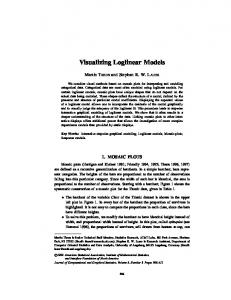
error rate is high, using more hypotheses supplies more ASR information to the dialogue act classifier, and thus improves the overall performance. Interestingly, although W1 and P1 both contain features from only one short utterance, sparse models are still able to remove the noisy features to improve the performance significantly. Here we see that the improvement of sparse models over MLR with WN is greater than with W1 , because using N -best hypotheses allows the sparse models to make use of more information. On the other hand, even though the phone n-gram feature set is denser than word n-gram, we are able to observe good results after applying sparse models for both 1-best and N -best hypotheses. 4.1.2. Word N -Gram and Phone N -Gram In Table 4, it is shown that word n-gram result of the MLR model is slightly better than phone n-gram for both 1-best and N -best lists, where n = [1...3]. Note that using N -best lists largely increases the dimension of word n-gram feature space, whereas the dimension of phone n-gram has only grown from 5,607 to 9,805. This reveals PN has a denser feature space. However, when using our sparse loglinear models, both WN and PN features have obtained significant improvements over MLR baseline, which demonstrates the robustness of our sparse models to filter noisy features in the settings with distinct dimentionalities. Considering these two types of feature sets might be additive, by combining WN and PN , Table 4 shows that using both feature sets results in better performance than using them separately. 4.1.3. Combining N -Gram and Confusion Networks CNet includes the features from the lattice of all hypotheses generated by a speech recognizer and dialogue context features [25, 36], which performs better than all n-gram feature sets. Combining WN , PN , and CNet further improves the performance, probably because phone n-grams provide additional information that CNet does not contain. In addition, non-sparse standard MLR using combined feature sets achieves a classification accuracy of 81.46%, whereas the best sparse model further improves the performance to 84.54%. The selected feature size is approximately 1% of original size. 4.2. Comparing MLR, Lasso, Ridge, and Elastic Net For the lasso model and the elastic net model, higher λ results in a sparser feature space, and we set λ1 = λ2 in the elastic net model to balance the same level of sparsity and smoothness. Models that are significantly better (P < 0.05) than the baseline are marked with asterisks in Table 4. We find that introducing penalty for larger weights in the standard MLR model has significant gains of 2%6%. The elastic net model balances the sparsity and smoothness and performs the best for most of the experimental settings. 4.3. Impacts of Different Levels of Sparsity Regularization parameters λ control the sparsity of the lasso and elastic net models. By showing the 3-fold cross-validation accura-

cies with different regularization parameters in Figure 1, we can see how the level of sparsity influences the performance. We find the performance from three models become better when increasing λ, clearly showing that penalizing features with large weights is useful. The accuracies for lasso model and elastic net model increase faster than ridge, because they encourage sparsity in the feature space and directly remove noisy features. Overall, they obtain better results than the ridge estimator. The elastic net model performs best and reaches the highest accuracy when smaller regularization parameters, since it balances sparsity and smoothness properly. ACC (%) 82

classes (occurrence > 3% in the test set) in Table 7. We find that the “null” and “hello” classes are difficult to classify, and here we show some examples of these dialogue acts:

81.5 81

• null: “uh”, “please” • hello: “hi i’m looking for a chinese restaurant please”, “hello i want italian restaurant in the south with moderate price”

80.5 80 79.5

79

Table 6. Classification accuracy using proposed models and other models. Results are written as µ ± 1.96σ, where µ is the estimate of mean over the utterances in the test set and σ is the standard error. Model Feature Accuracy (%) Phoenix manual grammar 70.6 ± 1.28 SVM 81.7 ± 1.08 MLR CNet 80.3 ± 1.12 Best Sparse MLR 84.1 ± 1.03 SVM 82.7 ± 1.06 MLR WN + PN + CNet 81.5 ± 1.09 Best Sparse MLR 84.5 ± 1.02

Lasso Ridge Elastic Net

0.2 0.4 0.6 0.8 1.0 1.2 1.4 1.6 1.8 2.0 2.2 2.4 2.6 2.8 3.0 λ

Fig. 1. Impacts of different levels of sparsity on 3-fold crossvalidation accuracy of the training set. 4.4. Comparing Element-Wise, Structured, and Hierarchical Sparse Models We compare element-wise, structured, and hierarchical sparse models for this task in Table 5. Here we use WN + PN + CNet and label these three feature sets as different groups to train group-wise sparse models. We find that group lasso doesn’t improve the performance, probably because we have not performed the exhaustive search to tune the parameters λm for different groups, since currently there might not exist efficient searching algorithms for tuning large number of group regularization parameters. Interestingly, the structured sparsity model using L1,∞ provides better result, revealing the importance of modeling sparsity structures. The hierarchical sparsity model that incorporates lasso and group lasso doesn’t give significant improvement, and possibly because this method has double L1 penalties, which hurts the performance when the model is too sparse. Table 5. Classification accuracy of testing set using element-wise, structured, and hierarchical sparse models. Model Accuracy (%) Element-wise Lasso 84.29 Group Lasso 83.39 Structured L1,∞ 84.41 Hierarchical Sparse Group Lasso 83.35 4.5. Comparing to Rule-based and Discriminative Models We compare our sparse models to Phoenix, which is the baseline that uses hand-crafted grammars [40], and SVM, which uses a linear kernel and sigmoid function to estimate the posterior probability for each class [41, 25]. Using the same feature set (CNet), our sparse MLR model significantly outperforms the linear kernel SVM model. Our proposed sparse model trained on the combined feature sets obtains the best performance. 4.6. Error Analysis and Discussion We perform an error analysis to understand where and why our models made mistakes. We show the accuracy for the six most frequent

Since “null” contains only very few words in an utterance and these words can also occur in other more frequent dialogue acts, estimating the parameters of these words in the classifier might be difficult. We might need the utterance length as a feature to capture this nuance. Also, the dialogue act “hello” hinges on the opening words in the utterance, but the rest of the words may confuse the classifier. This suggests that we might need to use the initial word as a feature in the future. Nevertheless, sparse models can still slightly improve the performance of these classes compared to non-sparse models. Table 7. Classification accuracy for the six most frequent classes. Class Ratio MLR Lasso Ridge Elastic Net inform 43.57% 88.11 92.81 92.38 93.14 request 25.13% 88.26 89.49 90.30 89.98 bye 13.72% 90.30 93.88 92.09 93.58 null 5.59% 49.08 49.45 50.92 49.45 hello 3.56% 35.63 36.78 38.51 37.36 affirm 3.48% 79.41 82.35 80.59 81.76 5. CONLUSION AND FUTURE WORK Sparse log-linear models improve dialogue act classification: we have observed absolute improvements over several baselines and a state-of-the-art SVM model are from 2.2% to 19.7%, and these improvements are robust across different feature and parameter settings. We find sparse models have larger gains on the word-level N best ASR hypotheses than that on the 1-best hypothesis, and when augmenting the word-level n-gram and confusion network features with phonetic features in our sparse models, we obtained the best performance in our dialogue act classification task. Empirical results show that the elastic net model that balances sparsity and smoothness obtains the best overall performance, while the L1,∞ structured sparsity model yields promising results among structured and hierarchical sparse models. Our error analysis shows that there is still room for improving the sparse models. Whilst his paper focuses on modeling textual outputs from ASR, sparse models can also be considered for modeling front-end features such as MFCC. In the future, we would like to investigate parameter sweep techniques for structured and hierarchical sparsity models. 6. ACKNOWLEDGEMENT We thank Matt Henderson for providing the data, and anonymous reviewers for useful comments.

7. REFERENCES [1] Jason D. Williams and Steve Young, “Partially observable Markov decision processes for spoken dialog systems,” Computer Speech and Language, 2007. [2] J. F. Allen, B. W. Miller, E. K. Ringger, and T. Sikorski, “A robust system for natural spoken dialogue,” in ACL, 1996. [3] W. Y. Wang and J. Hirschberg, “Detecting levels of interest from spoken dialog with multistream prediction feedback and similarity based hierarchical fusion learning,” in SIGDIAL, 2011. [4] H. Alshawi, “Effective utterance classification with unsupervised phonotactic models,” in NAACL-HLT, 2003. [5] Q. Huang and S. Cox, “Task-independent call-routing,” Speech Communication, 2006. [6] W. Schuler, S. Wu, and L. Schwartz, “A framework for fast incremental interpretation during speech decoding,” Computational Linguistics, 2009. [7] W. Y. Wang, R. Artstein, A. Leuski, and D. Traum, “Improving spoken dialogue understanding using phonetic mixture models,” in FLAIRS-24, 2011. [8] A. Chotimongkol and A. I. Rudnicky, “N-best speech hypotheses reordering using linear regression,” in EuroSpeech, 2001. [9] D. Hakkani-T¨ur, F. B´echet, G. Riccardi, and G. Tur, “Beyond ASR 1-best: Using word confusion networks in spoken language understanding,” Computer Speech & Language, 2006. [10] S. Yaman, L. Deng, D. Yu, Y.Y. Wang, and A. Acero, “A discriminative training framework using n-best speech recognition transcriptions and scores for spoken utterance classification,” in ICASSP, 2007. [11] E. Shriberg, A. Stolcke, D. Hakkani-T¨ur, and G. T¨ur, “Prosody-based automatic segmentation of speech into sentences and topics,” Speech communication, 2000. [12] R. Fernandez and R.W. Picard, “Dialog act classification from prosodic features using support vector machines,” in Speech Prosody, 2002. [13] J. Ang, Y. Liu, and E. Shriberg, “Automatic dialog act segmentation and classification in multiparty meetings,” in ICASSP, 2005. [14] V. K. Rangarajan Sridhar, S. Bangalore, and S. Narayanan, “Combining lexical, syntactic and prosodic cues for improved online dialog act tagging,” Computer Speech & Language, 2009. [15] D. Jurafsky, R. Bates, N. Coccaro, R. Martin, M. Meteer, K. Ries, E. Shriberg, A. Stolcke, P. Taylor, V. Ess-Dykema, et al., “Automatic detection of discourse structure for speech recognition and understanding,” in ASRU, 1997. [16] M. Zimmerman, D. Hakkani-T¨ur, J. Fung, N. Mirghafori, L. Gottlieb, E. Shriberg, and Y. Liu, “The ICSI+ multilingual sentence segmentation system,” in Interspeech, 2006. [17] R. Schwartz, S. Miller, D. Stallard, and J. Makhoul, “Language understanding using hidden understanding models,” in InterSpeech, 1996. [18] Esther Levin and Roberto Pieraccini, “CHRONUS, the next generation,” in Proc. of the DARPA Speech and Natural Language Workshop, 1995. [19] A. Stolcke, K. Ries, N. Coccaro, E. Shriberg, R. Bates, D. Jurafsky, P. Taylor, R. Martin, C.V. Ess-Dykema, and M. Meteer, “Dialogue act modeling for automatic tagging and recognition of conversational speech,” Computational linguistics, 2000. [20] A. Acero and Y. Y. Wang, “Spoken language understanding,” IEEE Signal Processing Magazine, 2005. [21] Y. He and S. J. Young, “Spoken language understanding using the hidden vector state model,” Speech Communication, 2006.

[22] M. Zimmermann, “Joint segmentation and classification of dialog acts using conditional random fields,” in INTERSPEECH, 2009. [23] S. Hahn, M. Dinarelli, C. Raymond, F. Lef`evre, P. Lehnen, R. De Mori, A. Moschitti, H. Ney, and G. Riccardi, “Comparing stochastic approaches to spoken language understanding in multiple languages,” IEEE TASLP, 2011. [24] P. Haffner, G. Tur, and J.H. Wright, “Optimizing svms for complex call classification,” in ICASSP, 2003. [25] M. Henderson, M. Gaˇsi´c, B. Thomson, P. Tsiakoulis, K. Yu, and S. Young, “Discriminative spoken language understanding using word confusion networks,” in SLT, 2012. [26] C. Chelba, Milind Mahajan, and Alex Acero, “Speech utterance classification,” in ICASSP, 2003. [27] U. Guz, G. Tur, D. Hakkani-T¨ur, and S. Cuendet, “Cascaded model adaptation for dialog act segmentation and tagging,” Computer Speech & Language, 2010. [28] Narendra Gupta, Gokhan Tur, Dilek Hakkani-T¨ur, Srinivas Bangalore, Giuseppe Riccardi, and Mazin Gilbert, “The AT&T spoken language understanding system,” IEEE Transactions on Acoustics, Speech and Signal Processing, 2006. [29] J. Eisenstein, N. A. Smith, and E. P. Xing, “Discovering sociolinguistic associations with structured sparsity,” in NAACLHLT, 2011. [30] W. Y. Wang, S. Finkelstein, A. Ogan, A. W. Black, and J. Cassell, ““love ya, jerkface”: using sparse log-linear models to build positive (and impolite) relationships with teens,” in SIGDIAL, 2012. [31] W. Y. Wang, E. Mayfield, S. Naidu, and J. Dittmar, “Historical analysis of legal opinions with a sparse mixed-effects latent variable model,” in ACL, 2012. [32] R. Tibshirani, “Regression shrinkage and selection via the lasso,” Journal of the Royal Statistical Society, Series B, 1994. [33] S. le Cessie and van J. C. Houwelingen, “Ridge estimators in logistic regression,” Applied Statistics, 1992. [34] H. Zou and T. Hastie, “Regularization and variable selection via the elastic net,” Journal of the Royal Statistical Society, Series B, 2005. [35] S. Young, “CUED standard dialogue acts,” Tech. Rep., Cambridge University Engineering Department, 2007. [36] L. Mangu, E. Brill, and A. Stolcke, “Finding consensus among words: lattice-based word error minimisation,” Computer Speech & Language, 2000. [37] M. Yuan and Y. Lin, “Model selection and estimation in regression with grouped variables,” Journal of the Royal Statistical Society Series B, 2006. [38] B. A. Turlach, W. N. Venables, and S. J. Wright, “Simultaneous variable selection,” in Technometrics, 2005. [39] J. Friedman, T. Hastie, and R. Tibshirani, “A note on the group lasso and a sparse group lasso,” Tech. Rep., Department of Statistics, Stanford University, 2010. [40] W. Ward, “Extracting information from spontaneous speech,” in InterSpeech, 1994. [41] J. Platt, “Probabilistic outputs for support vector machines and comparisons to regularized likelihood methods,” Advances in large margin classifiers, 1999.