An empirical model of TCP performance Allen B. Downey∗ Technical Report TR-2003-001 Olin College August 2003
Abstract
only steady-state behavior of TCP. Our model includes slow start and three steady-state behaviors: congestion avoidance, buffer-limited, and self-clocking. Two recent papers also consider buffer-limited steady state [2][14]; as far as we know, no other models include a self-clocking steady state. One limitation of many previous models is that they treat the drop rate as exogenous; that is, a characteristic of the network that is independent of the behavior of TCP. For many network paths, an important determinant of TCP performance is the occurrence of endogenous drops, which are caused by the transfer itself. Misra and Ott consider the case where loss probability depends on the congestion window [23]. Because of the complexity of this issue, our model abstracts away exogenous and endogenous drop rates. Instead, we estimate the probability of dropping out of slow start as a function of the current window size. Some models of short TCP transfers have been proposed [9][22][4][33][32]. These models identify two sources of variability in transfer times: variability in rtts and dropped packets. Our datasets suggest a third source of variability: nondeterminism in the growth of the congestion window during slow start. In some cases, this nondeterminism is the primary source of variability. We incorporate this behavior in our model. Another limitation of these models is that they do not address the transition from slow start to steady state (one exception is [13]). For many paths in the current Internet, this transition happens in the size range from 10–100KB, which happens to be the size range of many TCP transfers. In traces of Web downloads at Anonymized University, this range contained 15–20% of the transfers (based on our analysis of datasets from [5]). Thus, one contribution of this work is a model that includes all features that, according to observation, have a significant effect on TCP performance, including slow start, the transition to steady state, and all three steady-state behaviors. Of course, the price of completeness is complexity. Our model has more parameters than others, and it is based on details of a specific path, which requires a measurement infrastruc-
We propose a model of TCP performance that captures the behavior of a set of network paths with diverse characteristics. The model uses more parameters than others, but we show that each feature of the model describes an effect that is important for at least some paths. We show that the model is sufficient to describe the datasets we collected with acceptable accuracy. Finally, we show that the model’s parameters can be estimated using simple, application-level measurements.
1
Introduction
The goal of this work is to explore the feasibility of predicting TCP performance by (1) using measurements to estimate the characteristics of a network path, and (2) using a model of TCP and the estimated parameters to generate predictions. We would like to find a minimum-cost set of measurements that are sufficient to make acceptable predictions. Our approach is empirical in the sense that the model should include all features that affect performance in current networks. Thus we are forced to deal with the full diversity of Internet paths and hosts, including some unexpected phenomena; for example, we find that the growth of the congestion window during slow start is nondeterministic, at least for some sender-receiver pairs. A number of models have been proposed that relate TCP performance to various path characteristics, including round trip time, drop rate and bottleneck bandwidth. Most of these models focus on the steady state behavior of long transfers [15][19][20][27][21][29][28][24][11]. Because these models omit slow start, they cannot predict the performance of transfers where slow start makes up a significant part of transfer time, which are the vast majority of transfers. Also, they are based on the assumption that congestion avoidance is the ∗ Olin College of Engineering, Needham, MA 02492, email:
[email protected], web: www.allendowney.com
1
ture. But we show that this complexity is necessary; that is, it is impossible to make accurate predictions without it. We also show that the model is sufficient to describe the behavior of the datasets we collected, with two exceptions. Finally, we show that the network characteristics the model uses can be estimated from simple application-level measurements. Another contribution of this work is that our measurements reveal two phenomena that occur in real networks and that have a strong effect on TCP performance: self-clocking steady state (Section 2.1) and nondeterministic slow start (Section 3.3).
1.1
The answer to the second question depends on the application. In distributed environments, the available resources (computers, other devices, and the network links that connection) are known, and performance characteristics may be available. For example, the Network Weather Service (NWS) runs constantly in a Grid environment, monitoring the performance of a set of links and making reports available to applications. The techniques we propose here could be used in this kind of environment to collect data and make predictions. For HTTP and other TCP transfers, it is less obvious that the data needed to make a prediction are available. Users navigate the Web unpredictably, making transfers from many servers along many network paths. To investigate the feasibility of predicting HTTP transfers, we looked at logs collected by WWW proxy servers at Boston University in April and May 1998. These logs are available from the Internet Traffic Archive (http://ita.ee.lbl.gov/). Although users access many different servers, a small number of servers handle a significant part of the traffic. For example, the top-ten servers handled 30% of the requests. This observation suggests that a new request is likely to access a server that has been accessed many times in the past. To quantify this observation, we ran through the trace sequentially and, for each request, counted the number of times the same server had been accessed prior to the request. For the majority of accesses (63%), the history of previous accesses includes at least 30 requests. For a larger majority (81%) the history includes at least 10 requests. Access patterns in other environments show similar patterns. The LBL-CONN-7 dataset contains traces of more than 700,000 TCP connections between Lawrence Berkeley Laboratories and the rest of the Internet, recorded over 30 days in 1993. Of these, we extracted the 694,594 connections that transferred a known, nonzero amount of data. These connections access 12,657 unique IP addresses, but again the top-ten addresses handled 32% of the connections. For each connection we counted the number of connections to the same address that came before. In this case, a large majority of connections (81%) enjoy a history that includes at least 30 connections. Assuming, then, that the historical information we need is available, how much space would be necessary to maintain it? Based on the LBL dataset, we can imagine keeping data about 20,000 remote hosts. As an upper bound, we might keep data from the most recent 100 connections per host, and we expect most connections to transfer fewer than 100,000 bytes (in the BU dataset, only 0.3% of transfers are bigger). Such a history would require about 32 KB per host, or a total of 625 MB. We conclude that it is feasible to maintain a database
Applications
Why is it useful to predict the performance of TCP transfers? One reason is to improve user interfaces. For example, many web browsers display information on the progress of long transfers and make simple estimates of the remaining transfer times. In theory, these estimates are useful to users, but in current practice they are so inaccurate that many users have learned to ignore them. Another reason is to automate selection when a file is available from multiple servers. Often users are asked to choose among mirror sites based on geographic proximity, without information about the expected performance of the various paths. Finally, for distributed applications, predictions are useful for both resource selection and scheduling. Because network performance is so variable, it is usually impossible to predict the duration of a single transfer accurately. The best we can do is to provide a range or distribution of values. Thus, all of our predictions are stochastic, in the sense that we predict the distribution of transfer times, and evaluate the quality of prediction by the agreement of the predicted and actual distributions. These distributions can characterize sources of short-term variability, like queue delays, as well as sources of long-term variability, like path changes. Another application of our model is performance debugging. For many of the paths we observe, our analysis indicates which of several factors limit performance— bandwidth, congestion, slow start overhead, buffer capacity, etc. This information could be used for system tuning; for example, allocating buffer space at a busy server.
1.2
Availability of data
Our problem formulation is based on the assumption that when we predict the duration of a transfer, we know something about the network path the transfer will use, including the end points. The goal of this paper is two ask both “What information do we need?” and “What information can we expect to have?” 2
server 7 timing chart
with traces of previous TCP connections, and that for most of the paths a client uses, the database would contain information about a useful number of previous connections (10–30).
80
size (1000 B)
2
100
Measurement
There are three general approaches to network measurement. One is to collect packet-level information somewhere in a network path. Another is to collect kernel-level information at either the sender or receiver. The third is to collect information at the application level. The packet and kernel-level approaches provide the most detailed information and the most accurate timings. Application-level measurements are easy to implement, and the resulting tools are portable. We use application-level measurement to develop and evaluate our model. The analysis we use to estimate the model’s parameters and make predictions is also applicable to passive, network-level observation of TCP connections, but we find that the information we need is available at the application level, or can be inferred. Furthermore, in cases where timing inaccuracy is introduced, for example by context switches, these errors can be filtered out. In general, the variability in wide-area networks necessitates repeated measurement. This redundancy also mitigates the inaccuracy of applicationlevel measurement. Therefore, we expect the improvement from kernel- or network-level measurements to be small. Most Web browsers already contain code to monitor the progress of HTTP transfers. With a few small changes, we instrumented a version of GNU’s wget (available from gnu.org/software/wget) to record the arrival time of each chunk of data as presented to the application level. The following pseudocode shows the structure of the instrumentation:
60 40 20 0
0
100
200 300 time (ms)
400
500
Figure 1: Timing charts for 30 HTTP transfers.
on the arrival of packets and the ability of the OS to present packets to the application layer. In most cases, the spacing of packets is big enough that each read corresponds to one packet arrival. For each transfer, the modified version of wget produces two vectors: ti is the time in ms when the ith read started, and si is the total number of bytes read when the ith read completed. Figure 1 plots 30 transfers of a file from a Web server, showing s versus t. At the beginning of each transfer, the slow start mechanism is apparent. Increasing bursts of packets arrive at regular intervals. Looking at the number of packets in each burst, which we call the apparent window size, we infer that the congestion window at the sender doubles during each round, from 2 to 4 to 8. Looking at the intervals between bursts, we can make multiple estimates of the rtt. In the next round, we expect the congestion window to be 16, and in some cases there is a clear break after the 16th packet, but in many cases there is no apparent break, and packets arrive continuously at intervals of roughly 1.6 ms. These cases demonstrate successful TCP self-clocking (see Section 2.1). A few transfers show evidence of packet loss. When a packet is dropped, the OS can’t present additional data to the application layer until the retransmission arrives, so a drop appears as a long horizontal line. When the retransmission arrives, it is made available along with all the data that arrived in the interim; this mass “arrival” appears as a long vertical line. This path shows a significant number of drops, but in most cases they have little effect on performance. At the top of the figure, there are several transfers that suffer long delays because one of the last packets in the transfer was dropped. In this case, there are not enough duplicate ACKs to trigger Fast Retransmission; instead the sender waits for a timeout, with a significant impact on performance. This figure suggests a tentative list of the parameters
set the timer connect (socket) record elapsed time write (request) while (more data) { select (socket) record elapsed time read (buffer) record amount of data } The connect system call returns when the connection is established, so the first elapsed time is the time to send a SYN packet and receive a SYN-ACK packet. The select system call returns when data from the socket is available. The second elapsed time is the time to send a request and receive the first byte of the reply. For subsequent reads, the elapsed time depends 3
t = 0, cw = 8
R
Allman and Paxson claim “For TCP, this estimate is currently made by exponentially increasing the sending rate until experiencing packet loss” [1]. Barakat and Altman write “Due to the fast window increase, [slow start] overloads the network and causes many losses” [4]. In many common circumstances, these claims are incorrect on two counts:
S
t = 8, cw = 16
R
S
• The congestion window does not increase exponentially until a drop occurs. The double-per-rtt heuristic only applies until cw > bdp. After that, the rate of growth of the congestion window is limited by the arrival of ACKs, which is limited by the rate of data through the bottleneck. Until a drop occurs or cw exceeds ssthresh, the congestion window grows linearly with a slope of bdp/rtt = bw.
t = 10, cw = 16
R
S
• Slow start does not necessarily induce a drop. If there is enough buffer capacity in the network (quantified below), transfers can and often do transition into self-clocking steady state without inducing a drop.
Figure 2: Transition from slow start to self-clocking. that determine TCP performance: • Size and variability of rtt.
The following example and analysis explain these conclusions. Figure 2 shows the transition from slow start to self-clocking for a hypothetical network path, represented by a pipeline with bdp = 10 packets and a queue that drains 1 packet per time step. The queue represents the router before the bottleneck link in the path. Given bdp and the initial congestion window, we define cw∗ as the largest slow start congestion window smaller than bdp. In the example, cw ∗ = 8 packets. After the sender transmits these 8 packets, we define as t = 0 the moment before the first ACK reaches the sender. As each packet arrives, the sender increases cw and transmits two packets. Thus, at t = 8, cw = 16 and 8 packets have accumulated in queue. During the next two time steps, the queue drains slightly, and then the system reaches self-clocking steady state. During each time step, the congestion window increases by 1, the sender transmits 2 packets, the receiver gets 1 packet, and the queue grows by 1 packet. During each rtt, cw increases by bdp. Even though the sender is in slow start, the congestion window grows linearly. This pattern continues until a packet is dropped or cw exceeds ssthresh. In either case, the sender drops into congestion avoidance. In congestion avoidance, the congestion window grows more slowly, adding only one packet for each cw ACKs. Since the rate of growth is proportional to 1/cw, the congestion window grows logarithmically. The queue grows slowly, too; as long as the router at the bottleneck link has the capacity to store the queue, and there are few exogenous drops, self-clocking can continue. Even if a packet is dropped, self-clocking can
• Initial and subsequent congestion windows. • Bottleneck bandwidth. • Buffer size at the sender and receiver. • Frequency and performance impact of drops. • Steady-state behavior and throughput. In Section 3 we present techniques for estimating these parameters from measurements. The next two sections discuss self-clocking and buffer-limited steady state behavior. Timing diagrams for our datasets are available at allendowney.com/research/tcp/timing, along with our characterization of each.
2.1
Self-clocking
Conventional wisdom holds that the TCP slow start mechanism inevitably ends when the congestion window exceeds the bandwidth-delay product (bdp) and the sender induces one or more drops at the bottleneck link. As motivation for TCP Vegas, Brakmo and Peterson claim that TCP “needs to create losses to find the available bandwidth,” and later, “if the threshold window is set too large, the congestion window will grow until the available bandwidth is exceeded, resulting in losses . . . ” [8]. Similar claims are common in discussions of TCP performance: Hoe writes “. . . the sender usually ends up outputting too many packets too quickly and thus losing multiple packets in the same window” [16]. 4
server 2 timing chart
continue as long as cw doesn’t drop below bdp long enough to drain the queue. In some of our datasets, we observe exactly this behavior. The definitive characteristic of self-clocking steady state is that the rate-limiting factor is the bottleneck bandwidth, not the congestion window. During self-clocking, the sender may be in slow start or congestion avoidance, and the congestion window may be growing exponentially, linearly, or logarithmically. How much buffer capacity is needed? During the transition to self-clocking, the queue grows to cw ∗ packets and then shrinks to 2cw ∗ − bdp. In steady state, the queue grows again until cw = ssthresh, at which point the queue contains ssthresh − bdp packets. At that point the sender switches to congestion avoidance and the queue grows almost negligibly, adding one packet per cw time steps. In the best case, when ssthresh = bdp, this switch happens when the queue is only bdp − cw ∗ , which is less than bdp/2. This analysis is applicable if there are no exogenous drops during slow start, and if the perturbations caused by cross-traffic are small compared to the transmission time of a packet at the bottleneck. In that case the ACK stream will seldom be compressed, and the sender will seldom be induced to transmit faster than bw for more than two packets. This leaves us with an empirical question: how often does the transition to self-clocking succeed? Unfortunately, our observations are limited; in 10 of our 13 datasets, there is no opportunity to observe the transition because cw never reaches bdp. But the other three datasets (Servers 7, 9 and 10) suggest that self-clocking is common. For servers 7 and 10, the vast majority of transfers make the transition with no indication of dropped packets. For Server 9 about half of the transfers enter self-clocking; the other half enter congestion avoidance. These observations indicate that in many cases the self-clocking mechanism is effective, and that concerns about congestion induced by slow start may be overstated.
2.2
100
size (1000 B)
80 60 40 20 0
0
20
40 60 time (ms)
80
Figure 3: Timing charts for 30 HTTP transfers. information, T-RAT observes the advertised windown and uses heuristics to make this distinction [35]. This information is not available at the application level, but often the size of at least one of the buffers is. In our measurements, the receive buffer is large enough that it is never the limiting factor. Figure 3 shows a set of transfers where the ratelimiting factor is the send buffer. After 3 rounds of slow start, the apparent window size reaches 12 packets and doesn’t increase for the next four rounds. Since almost all transfers converge to the same window size, and most transfers show no sign of a drop, and the window size doesn’t increase, we infer that the limitation is the send buffer, not the congestion window.
3
The Datasets
Of course, a model of TCP performance should apply to the widest range of network conditions. To develop our model, we wanted to collect datasets from network paths with a variety of characteristics. The ubiquity and accessibility of Web servers makes them a convenient tool for network measurements. Two of our datasets come from servers provided by collaborators. The other 11 are popular servers we found in traces from the IRCache Project (http:// www.ircache.net/). Looking at one day of traces from 10 proxy servers, we identified frequently-accessed files that were at least 100,000 bytes. Starting with the most popular, we made measurements of the first 11 files we were able to download successfully. We used the HTTP/1.1 Range header to get only the first 100,000 bytes of data (plus roughly 350 bytes of header). Two servers ignored the Range header and sent the whole file. We chose a size of 100,000 bytes because we expected that most transfers of that size would leave slow start. In fact, we underestimated; in 6 of the datasets, most transfers never leave slow start.
Buffer-limited
In order to handle retransmissions, the sender has to keep a copy of all unacknowledged packets. Thus, the send buffer limits the amount of data in flight. Similarly, the receive buffer limits the advertised window, which limits the amount of data in flight. So the maximum sustained transmission rate is one buffer per rtt, where the limiting buffer is the smaller of the send and receive buffers. In general, it is not easy to tell whether the limiting factor is the send or receive buffer. Using packet-level 5
read lengths (cdf)
bandwidth estimates (cdf)
1.0
1.0
Pr (length < x)
0.8
Pr (bandwidth < x)
server 1 server 4 server 2
0.6 0.4 0.2 0.0
0
500
1000 x (bytes)
1500
0.8 0.6 0.4 0.2 0.0
2000
server 7 server 1 server 8
0
20
40 60 x (Mbps)
80
100
Figure 4: Cdf of read sizes for three servers.
Figure 5: Bandwidth estimates for three servers.
Each dataset includes 100 transfers, with an average of 100 seconds between them (exponential distribution). Thus, the duration of the measurements is 3–4 hours. This time scale is appropriate for our intended applications, where we expect historic information to be available, but not necessarily recent. The purpose of these datasets is to identify the parameters that determine TCP performance and to allow us to evaluate the model. A performance prediction tool would not need so much data, and it would not necessarily make active measurements. In fact, one advantage of this model is that it can work with passive measurements. The characteristics of the paths we measured are diverse. Geographical locations include New York, Chicago, Colorado, California, Maine, and China. The range of path lengths is from 12 to 29 hops. The range of rtts is from 7 to 270 ms. The range of bottleneck bandwidths is from 350 Kbps to 100 Mbps. The range of bdp is from 1 to almost 2000 packets. We believe that this dataset is representative of many paths in the current Internet. Our client is located at Boston University, which is a multi-hosted institution with relatively low-traffic, high-bandwidth network connections. So the client end of these paths may not be typical of Internet users. The following sections present the steps we used to process these datasets and estimate path characteristics. The heuristics we use are similar to those implemented in T-RAT, although T-RAT is based on packetlevel information [35].
read sizes for each server; Figure 4 shows three of them. Server 1 is typical of the servers we looked at; the other two are unusual. In the typical case, the vast majority of reads are 1448 or 1460 bytes, sizes that correspond to the maximum segment size (mss) of the path, minus L2 and L3 headers. For Servers 4 and 2, the most common read size is 1460 bytes, but a significant number of packets are smaller. The reason for this diversity is that the initial and subsequent congestion windows on this server are not integer multiples of the mss. We conclude that in most cases, the application is reading data fast enough to get a single packet per read, and that there are never more than two packets in the receive buffer.
3.1
3.2
Bottleneck bandwidth
The idea of using packet spacing to estimate bottleneck bandwidth was proposed by Keshav [17] and has been implemented in various network measurement tools [7][10][31][18][12]. Brakmo and Peterson implemented a version of TCP Vegas that uses packet-pair bandwidth estimates to choose the value of ssthresh [8]. Similar techniques have been proposed and evaluated elsewhere [16][3][1]. Partridge et al. have implemented a version of FreeBSD that uses packet pair estimates to accelerate slow start [30]. To implement packet-pair bandwidth estimation using our measurements, we compute the first difference of the vectors t and s, yielding dt, which is the interpacket spacing, and ds, which contains the packet sizes. For each packet, we compute the instantaneous bandwidth bwi = dsi /dti . If packets leave the bottleneck link back to back, and their spacing isn’t perturbed by cross traffic, bw estimates the bottleneck bandwidth of the path. Current bandwidth estimators are based on the assumption that packets often arrive at the destination with unperturbed packet spacing, and that the correct
Packet sizes
If the application reads data as soon as it is available, the data read usually correspond to single incoming packet. We expect that most applications can keep up with most wide-area networks, despite the vagaries of the local scheduler. To test this assumption, we plotted the distribution of 6
Server 1 2 3 4 5 6 7 8 9 10 11 12 13
bottleneck bandwidth is the mode of the distribution of estimates. Dovrolis et al. warn that under some traffic conditions, the global mode is determined by cross traffic and not bottleneck bandwidth, but they still expect a local mode at the correct value [12]. For continuous distributions, the notion of a mode is awkward to define, and methods for identifying modes tend to be ad hoc. Furthermore, many of our datasets exhibit no clear modes. Figure 5 shows distributions of bw estimates from servers with slow, medium and high bottleneck bandwidths. Server 7 shows a strong mode around 7 Mbps, but the other two cases are less promising. Server 8 shows a mode near 90 Mbps, but the distribution is nearly uniform from 70 to 100 Mbps. Similarly, the “mode” for Server 1 spans the range from 0 to 100 Mbps. It is difficult to generate a precise bandwidth estimate from these distributions. For our model, we have implemented a simple filtering technique that improves the repeatability of the bandwidth estimates, but we have not performed a rigorous evaluation of its accuracy. Fortunately, the model only needs a coarse estimate of the bandwidth. Bandwidth estimation based on TCP transfers is an active area of research; as improved methods become available, they can be incorporated into the model. Fortunately, we have more information to work with. Looking at timing charts like Figure 1, we see that interpacket spacing is highly variable, but there are many parallel linear segments that indicate a common slope. We assume that this characteristic slope corresponds to the bottleneck bandwidth, and try to estimate it statistically. Again, we start by computing, for each chart, the vector of bandwidth estimates bwi . For each of these vectors, we look at each subsequence of k bandwidth estimates, and compute the deviation of the jth subPj+k sequence, σj = 1/k i=j |bwi − m|, where m is the median of the estimates in the subsequence. The subsequences with the lowest deviation correspond to the straightest line segments in the timing chart. During processing, we keep only the n subsequences with the lowest deviation. We filter out the subsequences with higher deviation on the assumption that the packets were not sent back-to-back, or their interpacket spacing has been perturbed. Figure 5 (bottom) shows distributions of the estimates that remain after filtering with k = 8 and n = 100. In all three cases, the range of the estimates has been greatly reduced. Furthermore, in all of our datasets, the mode of the distribution is at or near the median; thus, we use the median as our bandwidth estimate and the interquartile distance as an indicator of its precision. This filtering technique works well with a range of values for k and n, provided that the sender frequently transmits k packets faster than the bottleneck bandwidth.
Est bw 24.908 63.656 89.040 92.710 90.677 63.870 6.982 91.261 0.331 9.376 89.474 22.694 88.775
Range (24.908, 28.014) (63.656, 86.860) (88.996, 90.051) (91.975, 92.712) (89.628, 91.937) (41.590, 84.870) (6.914, 7.075) (91.261, 92.313) (0.331, 0.513) (9.356, 9.412) (89.444, 90.866) (21.129, 33.811) (88.775, 90.142)
Interquart 1.147% 0.701% 0.513% 0.269% 0.687% 11.974% 0.212% 0.190% 5.845% 0.126% 0.669% 15.300% 0.386%
Table 1: Bandwidth estimates for each dataset. Estbw is based on all 100 timing charts. Range contains the highest and lowest estimates from each subset of 20 charts. Interquart is one-half the interquartile distance, written as a percentage of the estimated bw.
For Server 7, we happen to know that the bottleneck link in the path is a 10 Mbps ATM PVC. The estimated bandwidth is 7.0 Mbps, which may be a good estimate of the data throughput of the link, discounted for protocol and link-level overhead. For most of our datasets, we don’t know the actual bottleneck bandwidths of the path, so we can’t evaluate the accuracy of these estimates. But by dividing our datasets into subsets, we can evaluate their repeatability. For each dataset, we generate 5 subsets with 20 randomly-chosen timing charts in each. We generate a bandwidth estimate for each subset, and compute the range and interquartile distance of the five estimates. Table 1 shows the results for all 13 datasets. In most cases, the range of estimates is small, which suggests that they are actually measuring the capacity of a link in the path. However, one weakness of our technique is that it might be fooled by what Dovrolis et al. call a “post-narrow capacity mode.” For Server 6, the range of estimates is quite wide. On further investigation, we found that this dataset contains three paths with different characteristics. Subsequent requests for the same URL are handled by different servers, due to changes in DNS information caused by a distributed content delivery mechanism like those used by Akamai Technologies and Speedera Networks. The filtering technique we use here can be integrated into existing bandwidth measurement tools. As future work, we plan to evaluate this technique more rigorously and compare it with existing tools. 7
server 7 window sizes
this threshold has little effect. As the congestion window approaches bdp, it becomes impossible to identify rounds, but fortunately it is unnecessary, because at that point we identify and characterize the steady-state behavior.
observed window (packets)
4 3 2 1
40 30
Figure 6(top) shows a server with the kind of slow start behavior we expect. The first round is always 2 packets, the second is always 4, and the third is usually 8, except in a few cases where, it seems, a drop causes the sender to switch to congestion avoidance. By the fourth round, the congestion window has reached bdp, which is about 15 packets, and it is no longer possible to identify the breaks between rounds accurately.
20 10 0
0
20
40 60 measurement
80
server 3 window sizes 4 3 2 1
observed window (packets)
15
Figure 6: Window sizes for the first four rounds of slow start, for 100 HTTP connections.
Although this behavior is comprehensible, it is not typical. In most of our datasets, the behavior of the congestion windows turns out to be nondeterministic. Figure 6(bottom) shows an example. The initial congestion window is consistently 2524 B, a little less than 2 packets. But the second round is sometimes 3 and sometimes 4 packets. The third round is usually twice the second, but again, it sometimes falls short by a packet or two. The same thing happens in the next round; the congestion window either doubles or nearly doubles, seemingly at random. Of our 13 datasets, 10 show significant nondeterminism starting in the second or third round and continuing in subsequent rounds.
3.3
The window sizes for all datasets are available from allendowney.com/research/tcp/wins.
10
5
0
0
20
40 60 measurement
80
Congestion windows
The most likely explanation of this behavior is an interaction between the delayed ACK mechanism at the receiver and the growth of the congestion window at the sender. In steady state, most receivers send one ACK for every two packets. Other ACKs are delayed until the next packet arrives or until a timer expires [26].
The duration of short TCP transfers tends to be a multiple of the round trip time, where the multiplier depends on the behavior of the congestion window at the sender. Thus, in order to predict TCP performance for a given server, we have to measure its initial and subsequent congestion windows. To do that, we have to be able to identify the end of each round of packets. To separate arriving packets into rounds, we look at the vector of interpacket spacing, ds, and identify intervals that seem to be due to congestion control rather than queue delays. To do that, it helps to know rtt and the interpacket spacing at the bottleneck. As a coarse estimate of rtt, we collect the measured rtts of the SYNACK and request-reply rounds and compute their 5th percentile. To get the interpacket spacing at the bottleneck, we use the bandwidth estimation technique in the previous section and compute, inter = dsi /bw. Then we compute a logarithmic transformation of the interarrival time, dt0i = f (dti ), scaled so that dt0i = 0 if dti = inter and dt0i = 1 if dti = rtt. This transformation gives us a criterion for breaking a timing chart into rounds; if dt0i > 0.5, we consider the ith packet to be the beginning of a new round. During slow start, the breaks between rounds are obvious and the choice of
During slow start, many senders increase the congestion window by one mss for each new ACK that arrives. If the receiver acknowledges every other packet, the congestion window tends to grow by a factor of 1.5 per round. To accelerate the growth of the congestion window, many receivers ACK every packet during slow start. In general, though, the receiver does not know whether the sender is in slow start and must use heuristics. In accordance with RFC1122, most receivers use a timer to bound the time an ACK is delayed. We suspect that this timer is the source of nondeterminism in window sizes. For our datasets, the receiver was running Red Hat Linux 7.3 (kernel version 2.4.18-3). On this system, the duration of the delayed ACK timer depends on the estimated rtt, with minimum and maximum values of 40 and 200 ms. 8
server 2 rtts (cdf)
syn-ack delays (cdf)
1.0 0.975 0.9
Pr (delay < x)
Pr (rtt < x)
0.8 0.6 0.4 syn-ack req-rep data
0.2 0.0
0.25
server server server server
0.025
7
10
14 x (ms)
19
-1
26
server 3 rtts (cdf)
0
1 x (log10 ms)
4 10 7 9
2
Figure 8: Distributions of delays for the SYN-ACK round, for four servers. The axes are transformed so that a lognormal distribution appears as a straight line.
0.8
Pr (rtt < x)
0.5
0.1
1.0
0.6
server is synchronous and may require disk access. In two of our datasets, the rtts for the request-reply round are 2–10 times longer than the network rtt. Figure 7(bottom) shows an example. Clearly for this kind of application, a model of TCP performance needs to include a model of application-level performance. After the request-reply round, the servers we observed seem to keep up with the network. Even in high-bandwidth, low-rtt paths, the subsequent data rounds happen at network speed. Server 3 is an exception. After the first 40 packets, each transfer is delayed by roughly 50 ms (a few are shorter and a few are as long as 400 ms). Since the distribution of these delays is nothing like the distribution of network rtts, we conclude that they are caused by the server, possibly the local scheduler. In general, though, our measurements do not distinguish between network and server delays. Barford and Crovella address this problem more successfully using network-level traces [6]. In general, the distribution of network delays is heavily skewed. Therefore, moments computed from samples do a poor job of characterizing the shape of the distribution. In many cases, the distribution of rtts is well-described by a three-parameter lognormal model. For a given set of measured rtti , we estimate the minimal value, θ = min rtti , and then compute the delays, delayi = rtti − θ. By plotting the distribution of delays, we can see whether the lognormal model is appropriate. Figure 8 shows the delays for the SYN-ACK round for four servers with a range of variability. The axes have been transformed so that a lognormal distribution appears as a straight line. The actual distributions are only approximately straight, but they are close enough that we think the lognormal parameters summarize them well. Table 2 shows the estimated parameters for the SYN-
0.4 syn-ack req-rep data
0.2 0.0
19
46
112 x (ms)
269
647
Figure 7: Distributions of round trip times for the SYNACK round, reply-request round, and next three data rounds of 100 HTTP connections.
3.4
0.75
Round trip time
For short transfers, the distribution of transfer times depends on the distribution of rtts. In general it is trivial to measure the rtt of a network path. Tools like ping can send packets of various types and sizes, and measure the time to get a reply. So it is no surprise that we can use TCP to estimate rtt, or that by making repeated measurements we can estimate the distribution of rtts. A TCP connection takes at least two rtts, one for the SYN-ACK round and one for the request-reply round. If the transfer size is greater than the initial congestion window, additional data rounds are required. In our datasets, we can measure the SYN-ACK and requestreply rounds directly, and after segmenting the timing chart we can estimate the rtts of the next three data rounds reliably. Figure 7 shows distributions of rtt for SYN-ACK, reply-request, and the first data round. Server 2 (top) is typical. The SYN-ACK round sees the shortest rtts because the packet sizes are minimal and there is no application-level processing at the server. The requestreply round takes the longest, and has the highest variability, because the application-level processing at the 9
Server 1 2 3 4 5 6 7 8 9 10 11 12 13
θ ms 271.564 7.351 14.247 75.239 6.648 6.611 24.471 87.689 37.593 50.942 227.368 239.564 50.225
ζ log10 ms 1.198 -0.379 -0.114 -0.547 -0.253 0.087 0.505 -0.414 1.452 0.009 1.218 1.960 -0.541
σ log10 ms 0.545 0.424 0.292 0.316 0.126 0.746 0.703 0.598 0.833 0.662 0.870 0.238 0.301
E[delay] ms 3.842 0.749 0.931 0.608 0.783 1.441 2.120 0.790 6.038 1.256 4.937 7.303 0.609
Server 1 2 3 4 5 6 7 8 9 10 11 12 13
syn-ack req-rep 0.203 (-0.113) (-0.082) (0.096) (0.116) 0.671 0.396 (0.044) 0.721 0.184 0.811 0.631 (-0.040)
req-rep data 1 0.180 (0.126) (-0.131) 0.265 (-0.121) 0.640 0.334 (-0.020) 0.682 (0.081) 0.745 0.625 (0.101)
data 1 data 2 0.220 (0.076) 0.702 (-0.034) (0.088) 0.736 0.310 (-0.185) 0.657 (0.157) 0.874 0.875 (-0.047)
data 2 data 3 0.364 (-0.108) 0.770 (-0.008) (0.092) 0.713 0.326 (-0.269) 0.638 (-0.144) 0.915 0.895 (-0.043)
Table 2: Estimated parameters for the distribution of rtts in the SYN-ACK round for 13 servers.
Table 3: Correlations in rtt for the first four rounds of TCP connections.
ACK round for each server. The parameters ζ and σ are the mean and standard deviation of log 10 delay. The expected value of delay is E[delay] = pow(10, (ζ + σ 2 /2)).
two rounds are insignificant because the duration of the request-reply round is limited by the server and unrelated to network conditions. Based on prior work, we might expect higher correlations on paths with shorter rtts, but that is not the case. There is no apparent relationship between rtt and the degree of correlation. On the other hand, paths with high expected delays (see E[delay] in Table 2) tend to have high correlations. This result makes sense, since paths with longer delays are more likely to have queues that persist long enough to induce correlations on the relevant time scale.
3.5
Correlations
The duration of a short TCP transfer is the sum of a series of consecutive rtts. Therefore, correlation between successive rtts affects the distribution of transfer times. In general the strength of correlation depends on the interval between packets. For modeling TCP performance, the relevant interval is the rtt of the path. Bolot characterized the relationship between the rtts of successive packets and found that correlations diminish as the timescale increases, and disappear when the interval between packets exceeds 500ms [7]. Moon et al. estimate the autocorrelation function for series of RTP packets and find strong correlations that diminish over larger intervals, again becoming insignificant beyond 500ms [25]. By breaking our observations of slow start into a series of rtts, we can use our measurements to estimate correlations between successive rounds. For each round, we compute the cdf of all rtts seen during that round. Then for each timing chart, we find the rank of each observed rtt in the cdf for its round. Next we transform the ranks using the inverse of the normal distribution function, and then compute Pearson’s correlation. Table 3 shows the estimated correlations for the first four rounds, for each server. Values in parentheses are statistically insignificant at 90% confidence. About half of the servers show significant correlations, some larger than 0.8. All significant correlations are positive, and usually consistent from round to round. For Server 3, the correlation between data rounds is above 0.7, but the correlations in the first
4
Performance model
Finally we are ready to assemble a model of TCP performance. The model is based on the following state transition diagram: ss0
ss1
ss2
ca
ssn
bl
sc
The states labeled ss0 through ssn are slow start states; the states labeled ca, bl and sc represent congestion avoidance, buffer-limited, and self-clocking steady state. By looking at the timing chart for each transfer, we try to identify the sequence of states the transfer went through. For each transfer, we have a series of observed window sizes, wi , computed as in Section 3.3. All transfers start in ss0. If w0 is less than 5.0, we move to ss1; a larger window probably indicates a dropped packet, so we move to ca. For subsequent rounds, we compute the 10
ratio of successive window sizes, wi /wi−1 . If this ratio is between 1.5 and 2.0, we move to the next slow start state. If it falls short of 1.5, we assume that a dropped packet caused the congestion window to shrink and we move to ca. If we see evidence of a dropped packet (see Section 2), we also move to ca. Finally, if the window exceeds bdp, we move to sc. For the slow start states and bl, we keep track of the distribution of window sizes in each state. For states ca and sc, we keep track of the distribution of throughputs, computed as the average throughput between the end of the last round of slow start and the end of the timing chart. Thus, for each timing chart, we compute a series of states that starts in ss0 and ends when the transfer ends or when it reaches one of the terminal states, ca and sc. By counting the state transitions in these series, we estimate the probability of each state transition. The states of the model describe the behavior of a transfer, and do not necessarily correspond to the TCP state of the sender or receiver. For example, when the model infers that a transfer is in self-clocking steady state, the sender might be in slow start or congestion avoidance. This is an abstraction, not an error. The model now contains all the information we need to compute the distribution of transfer times for a given size. By making a random walk through the state transition diagram, we can generate a single estimate of the transfer time. By making repeated walks, we can estimate the distribution. The next section explains this process in more detail.
4.1
ttotal , the total elapsed time, to rtt0 + rtt1 . Start in state ss0. 2. Using the state transition probabilities, choose the next state at random. 3. If the new state is ca or sc, choose throughput at random from the distribution of throughputs. Compute the remaining time trem = (s − stotal )/throughput and return the sum trem +ttotal . 4. Choose a window size, win, from the distribution of window sizes for the current state. If stotal +win > s, the transfer completes during this round. Return ttotal . 5. Update stotal = stotal + win. Choose rtt from the distribution of data rtts, and update ttotal = ttotal + rtt. 6. Go to step 2. By repeating this process, we estimate the distribution of transfer times.
5
Validation
To test the model, we divide each dataset randomly into two sets of 50 transfers. We use the first subset to estimate parameters and generate a distribution of transfer times for a range of sizes. Then we compare the predicted times with the measured times from the second subset. Figure 9 shows the results for four servers we chose to represent various steady state behaviors. For Server 1, most transfers end in slow start. For some file sizes, the distribution of transfer times is multimodal because the characteristics of the path changed during the measurement. The model captures this behavior well. For Server 2, most transfers are buffer-limited, so the transfer time is determined by the distribution of rtts. In this case the distributions are multimodal because the growth of the congestion window is nondeterministic. For Server 9, many transfers enter congestion avoidance almost immediately, but some are self-clocking. The range of transfer times is unusually wide, but the model describes the distributions reasonably well. For Server 10, most transfers are self-clocking and the range of transfer times is relatively narrow. Similar figures for all 13 datasets are available from allendowney.com/research/tcp/aptimes.100000. In two cases, the model is not as successful. As discussed in Section 3.4, transfers from Server 3 see a delay after the first 40 packets. Since this delay isn’t included in the model, our predictions for longer transfers are too short. The other problem is Server 6, which is actually
Estimating transfer times
In previous sections, we have shown how to use a set of timing charts to estimate the parameters of a network path. These parameters are: • The distribution of rtts for the SYN-ACK round, the request-reply round, and the first data round. • The correlation in rtts for the first two data rounds. • The state transition probabilities for n slow start states plus ca, sb and sc. • The distribution of window sizes for each slow start state, and bl. • The distribution of throughputs for ca and sc. These parameters are sufficient to estimate the transfer time for a given transfer size, s. Here is the algorithm in pseudocode: 1. Set stotal , the total data received, to 0. Choose rtt0 from the distribution of SYN-ACK rtts and rtt1 from the distribution of request-reply rtts. Set 11
Server 1 2 3 4 5 6 7 8 9 10 11 12 13
server 1 tts (cdf)
Pr (transfer time < x)
1.0 0.8 0.6 0.4
1000 5000 20000 50000 100000
0.2 0.0
563
1119
2227 x (ms)
4431
8815
server 2 tts (cdf)
Distance 100,000 0.804 0.771 3.490 0.087 2.639 3.682 0.937 0.265 1.938 1.194 1.237 0.782 0.697
Distance 50,000 1.044 3.475 8.716 0.303 1.871 6.802 0.627 0.459 2.194 2.023 2.657 0.803 2.254
Pr (transfer time < x)
1.0
Table 4: Distance metrics for predicted transfer times, given measurements truncated after 100,000 or 50,000 bytes.
0.8 0.6 0.4
1000 5000 20000 50000 100000
0.2 0.0
18
29
46 x (ms)
74
three servers with different path characteristics. Subsequent requests for the same URL are handled by different servers, due to changes in DNS information caused by a distributed content delivery mechanism like those used by Akamai Technologies and Speedera Networks. The model combines the characteristics of the three paths, forming a trimodal distribution of rtts. When we convolve this distribution with itself, it gets smoother, whereas the real distribution of transfer times is sharply trimodal. Although the location and variance of the predicted distribution are right, the shape is not. Although some servers exhibit features that are not captured by the model, the model is able to capture the behavior of a wide range of server and network conditions.
119
server 9 tts (cdf)
Pr (transfer time < x)
1.0 0.8 0.6 0.4
1000 5000 20000 50000 100000
0.2 0.0
121
419
1450 x (ms)
5011
17317
5.1
server 10 tts (cdf)
Pr (transfer time < x)
1.0
A stronger test of the model is whether, given measurements of short transfers, it can predict the duration of long transfers. To simulate measurements of shorter transfers, we cut off each timing chart after the first 50,000 bytes and predict the duration of 100,000 byte transfers. Again, we divide the datasets in half, using 50 timing charts to build the model and testing it on the other 50. Table 4 shows the results, comparing a distance metric for predictions that use the censored measurements (right column) with the predictions from the previous section (left column). Graphs of the predicted and actual distributions are available from allendowney.com/research/tcp/ aptimes.50000. The distance metric is, loosely speaking, the normal-
0.8 0.6 0.4
1000 5000 20000 50000 100000
0.2 0.0
119
245
504 x (ms)
1036
Short measurements
2130
Figure 9: Distributions of predicted (thick, gray lines) and actual transfer times (thin, darker lines).
12
6.1
ized area between the predicted and actual distributions, computed by summing for each percentile, p, from 1 to 99:
Application-level measurements are easy to implement, and tools that use them are portable. The price of this convenience is that some of the things we would like to measure, like drop rates and window sizes, are not directly visible to an application. We have shown that it is possible to infer this information with acceptable accuracy, but there are two parts of the model that would benefit from more network-level information. The first is identifying dropped packets. The heuristics our model uses are successful in the sense that they identify characteristics in a timing chart that indicate a dropped packet, but without network-level traces we can’t assess their accuracy. The second limitation is the difficulty of distinguishing server delays from network delays. For the HTTP transfers we looked at, most server delays occur during the request-reply round; after that, the servers kept up with the network. Other kinds of TCP transfers, like ftp, may be similar, but there are other cases where a more detailed model of server performance may be necessary. Finally, an aspect of TCP performance that we left out of the model is the effect of dropped packets at the end of a transfer. In our datasets, most drops were caught by the Fast Retransmit mechanism, so they tended not to impose long delays, except indirectly by reducing the congestion window. When a packet is dropped at the end of a transfer, there may not be enough ACK packets to trigger Fast Retransmit, and a transfer may suffer a timeout. In our datasets, these events are rare, but their effect is significant.
|Fp−1 (p) − Fa−1 (p)| Fa−1 (p) where Fp and Fa are the actual and predicted distribution functions. For most servers, the predictions based on censored data are good, either a little worse or, by chance, a little better than the predictions that use all the data. When the predictions fail it is because the truncated datasets don’t contain enough information to classify the steady-state behavior of the server. For example, Server 2 is buffer-limited, but in the truncated dataset it never leaves slow start, so the model predicts transfer times that are too short. We conclude that, in order to predict the performance of long transfers, it is critical to observe at least a few transfers that leave slow start.
6
Limitations
Conclusions
Using measurements from a small but diverse set of network paths, we identify the set of network parameters that are necessary to predict TCP performance, and show that these parameters can be estimated with a reasonable number of application-level measurements. We propose a model that uses estimated parameters to make stochastic predictions of TCP performance. The features of this model are: • It models slow start and three steady-state behaviors: congestion avoidance, buffer-limited, and selfclocking. Thus, it is applicable to the full range of transfer sizes.
6.2
• Rather than estimate the exogenous drop rate explicitly, the model incorporates both exogenous and endogenous drops in an array of state transition probabilities.
Future Work
Our experiments show that the parameters of the model are consistent; when we divide a dataset in half at random, we can use the parameters from one half to predict the performance of the other half. The next step is to make the model predictive; that is, given a set of past measurements, we would like to predict future performance. To do that, we have to address two additional problems. The first is to find a number of measurements, and their timescale, that is sufficient to capture the stochastic properties of a network path. The second is to identify and deal with the nonstationarity induced by path changes and other large-timescale variability. Fortunately, several previous projects have addressed these problems, including the Network Weather Service (NWS) [34]. Our next step is to incorporate our model into a measurement infrastructure like the NWS. Many thanks to Dhiman Barman, John Byers, Azer Bestavros and Mark Crovella at Boston University for enlightening conversations about this paper. Also
• The model includes correlations between successive rtts, which is important on paths where the expected queue delays are large compared to rtt. • It is applicable to all current and most conceivable implementations of TCP, provided that they implement Fast Retransmission. In some cases, its estimated parameters can be used to identify the implementation of the sender or receiver. Our measurements reveal two phenomena that are relevant to TCP performance. The first is that selfclocking may make TCP less prone to endogenous drops than previously believed. The second is that the growth of the congestion window during slow start is nondeterministic, at least for some TCP implementations. 13
thanks to K Claffy at CAIDA for all her help and support.
[13] N. Ehsan and M. Liu. Analysis of TCP transient behavior and its effect on file transfer latency. In IEEE ICC, May 2003.
References
[14] A. Fekete and G. Vattay. On buffer limited congestion window dynamics and packet loss. In IEEE Internet Performance Symposium, November 2002.
[1] M. Allman and V. Paxson. On estimating end-toend network path properties. In SIGCOMM, pages 263–274, 1999.
[15] S. Floyd. Connections with multiple congested gateways in packet-switched networks part 1: Oneway traffic. ACM Computer Communication Review, 21(5):30–47, Oct. 1991.
[2] E. Altman, K. Avrachenkov, C. Barakat, and R. N. nez Queija. TCP modeling in the presence of nonlinear window growth. Technical Report RR-4312, INRIA, Novemeber 2001.
[16] J. C. Hoe. Improving the start-up behavior of a congestion control scheme for TCP. In ACM SIGCOMM, pages 270–280, 1996.
[3] M. Aron and P. Druschel. TCP: Improving startup dynamics by adaptive timers and congestion control. Technical report, Dept. of Computer Science, Rice University, 1998.
[17] S. Keshav. A control-theoretic approach to flow control. In ACM SIGCOMM, pages 3–15, 1991. [18] K. Lai and M. Baker. Measuring bandwidth. In IEEE INFOCOM, pages 235–245, 1999.
[4] C. Barakat and E. Altman. Performance of short TCP transfers. In NETWORKING, volume 1815 of Lecture Notes in Computer Science, pages 567– 579. Springer, 2000.
[19] T. Lakshman and U. Madhow. The performance of TCP/IP for networks with high bandwidth-delay products and random loss. IEEE/ACM Transactions on Networking, 5(3):336–350, July 1997.
[5] P. Barford, A. Bestavros, A. Bradley, and M. Crovella. Changes in web client access patterns: Characteristics and caching implications. World Wide Web, Special Issue on Characterization and Performance Evaluation, 2:15–28, 1999.
[20] T. V. Lakshman, U. Madhow, and B. Suter. Window-based error recovery and flow control with a slow acknowledgement channel: A study of TCP/IP performance. In INFOCOM (3), pages 1199–1209, 1997.
[6] P. Barford and M. Crovella. Critical path analysis of TCP transactions. In SIGCOMM, pages 127– 138, 2000.
[21] M. Mathis, J. Semke, and J. Mahdavi. The macroscopic behavior of the TCP congestion avoidance algorithm. Computer Communications Review, 27(3), 1997.
[7] J.-C. Bolot. Characterizing end-to-end packet delay and loss in the internet. Journal of High Speed Networks, 2(3):289–298, September 1993.
[22] M. Mellia, I. Stoica, and H. Zhang. TCP model for short lived flows. IEEE Communications Letters, 6(2):85–88, February 2002.
[8] L. S. Brakmo and L. L. Peterson. TCP Vegas: End to end congestion avoidance on a global internet. IEEE Journal on Selected Areas in Communications, 13(8):1465–1480, 1995. [9] N. Cardwell, S. Savage, and T. Anderson. Modeling TCP latency. In INFOCOM (3), pages 1742– 1751, 2000.
[23] A. Misra and T. J. Ott. The window distribution of idealized TCP congestion avoidance with variable packet loss. In INFOCOM (3), pages 1564–1572, 1999.
[10] R. Carter and M. Crovella. Measuring bottleneck link speed in packet-switched networks. Technical Report TR-1996-006, Computer Science Dept., Boston University, 1996.
[24] V. Misra, W. Gong, and D. Towsley. Stochastic differential equation modeling and analysis of TCP windowsize behavior. Technical Report ECE-TRCCS-99-10-01, University of Massachusetts, 1999.
[11] C. Casetti and M. Meo. A new approach to model the stationary behavior of TCP connections. In INFOCOM (1), pages 367–375, 2000.
[25] S. B. Moon, J. Kurose, P. Skelly, and D. Towsley. Correlation of packet delay and loss in the Internet. Technical Report UM-CS-1998-011, University of Massachusetts, March 1998.
[12] C. Dovrolis, P. Ramanathan, and D. Moore. Packet dispersion techniques and capacity estimation. Submitted to IEEE/ACM Transactions in Networking.
[26] W. Noureddine and F. Tobagi. The transmission control protocol. Technical report, Stanford University, July 2002. 14
[27] T. Ott, J. Kemperman, and M. Mathis. Window size behavior in TCP/IP with constant loss probability. In IEEE HPCS, June 1997. [28] J. Padhye, V. Firoiu, and D. Towsley. A stochastic model of TCP Reno congestion avoidance and control. Technical Report CMPSCI 99-02, University of Massachusetts, 1999. [29] J. Padhye, V. Firoiu, D. Towsley, and J. Krusoe. Modeling TCP throughput: A simple model and its empirical validation. In ACM SIGCOMM, pages 303–314, 1998. [30] C. Partridge, D. Rockwell, M. Allman, R. Krishnan, and J. Sterbenz. A swifter start for TCP. Technical Report 8339, BBN, March 2002. [31] V. Paxson. End-to-end Internet packet dynamics. IEEE/ACM Transactions on Networking, 7(3):277–292, 1999. [32] B. Sikdar, S. Kalyanaraman, and K. Vastola. Analytic models for the latency and steady-state throughput of TCP Tahoe, Reno and SACK. In IEEE GLOBECOM, pages 1781–1787, November 2001. [33] B. Sikdar, S. Kalyanaraman, and K. Vastola. TCP Reno with random losses: Latency, throughput and sensitivity analysis. In IEEE IPCCC, pages 188–195, April 2001. [34] R. Wolski, N. T. Spring, and J. Hayes. The Network Weather Service: a distributed resource performance forecasting service for metacomputing. Future Generation Computer Systems, 15(5– 6):757–768, 1999. [35] Y. Zhang, L. Breslau, V. Paxson, and S. Shenker. On the characteristics and origins of internet flow rates. In SIGCOMM, 2002.
15