An Empirical Study of MDL Model Selection with Infinite Parametric

An Empirical Study of MDL Model Selection with Infinite Parametric Complexity

arXiv:cs/0501028v1 [cs.LG] 14 Jan 2005

Steven de Rooij and Peter Gr¨ unwald February 1, 2008

Abstract Parametric complexity is a central concept in MDL model selection. In practice it often turns out to be infinite, even for quite simple models such as the Poisson and Geometric families. In such cases, MDL model selection as based on NML and Bayesian inference based on Jeffreys’ prior can not be used. Several ways to resolve this problem have been proposed. We conduct experiments to compare and evaluate their behaviour on small sample sizes. We find interestingly poor behaviour for the plug-in predictive code; a restricted NML model performs quite well but it is questionable if the results validate its theoretical motivation. The Bayesian model with the improper Jeffreys’ prior is the most dependable.

1

Introduction

Model selection is the task of choosing one out of a set of alternative hypotheses, or models, for some phenomenon, based on the available data. Let M1 and M2 be two parametric models and D be the observed data. Modern MDL model selection proceeds by associating so-called universal codes (formally defined in Section 2) with each model. We denote the resulting codelength for the data by LM(D), which can be read as ‘the number of bits needed to encode D with the help of model M’. We then pick the model M that minimises this expression and thus achieves the best compression of the data. There exist a variety of universal codes, all of which lead to different codelengths and thus to different model selection criteria. While any choice of universal code will lead to an asymptotically ‘consistent’ model selection method (eventually the right model will be selected), to get good results for small sample sizes it is crucial that we select an efficient code. According to the MDL philosophy, this should be taken to mean a code that compresses the data as much as possible in a worst-case sense. This is made precise in Section 2. Whenever this code, known as the Shtarkov or NML code, is well-defined MDL model selection is straightforward to apply and typically leads to good results (see [12] and the various experimental papers therein). However, the worst-case optimal universal code can be ill-defined even for such simple models as the Poisson and geometric models. In such cases it is not clear how MDL model selection should be applied. A variety of remedies to this problem have been proposed, and in this paper we investigate them empirically, for the simple case where M1 is Poisson and M2 geometric. We find that some solutions, most notably the use of a plug-in code instead of the NML code, lead to relatively poor results. However, since these codes no longer minimise the worst-case regret they are harder to justify theoretically. In fact, as explained in more detail in Section 4.4, the only method that may have an MDL-type justification closely related to minimax regret is the Bayesian code with the improper Jeffreys’ prior. Perhaps not coincidentally, this also seems the most dependable code among all solutions that we tried.

1

In Section 2 we describe the code that achieves worst-case minimal regret. This code is undefined for the Poisson and geometric distributions. We analyse these models in more detail in Section 3. In Section 4 we describe four different approaches to MDL model selection under such circumstances. We test these using error rate and calibration tests and evaluate them in Section 5. Our conclusions are summarized in Section 6.

2

Universal codes

A universal code is universal with respect to a set of codes, in the sense that it codes the data in not many more bits than the best code in the set, whichever data sequence is actually observed. We thus define universal codes on an individual sequence basis, as in [2], rather than in an expected sense. The difference between the codelength of the universal code and the codelength of the shortest code in the set is called the regret, which is a function of a concrete data sequence, unlike “redundancy” which is an expectation value and which we do not use here. There exists a one-to-one correspondence between code lengths and probability distributions: for any probability distribution, a code can be constructed such that the negative logs of the probabilities equal the codeword lengths of the outcomes, and vice versa; here we conveniently ignore rounding issues [11]. Therefore we can phrase our hypothesis testing procedure in terms of statistical models, which are sets of probability distributions, rather than sets of codes. In this paper, we define universal codes relative to parametric families of distributions (‘models’) M, which we think of as sets of distributions or sets of code length functions, depending on circumstance. Let U be a code with length function LU . Relative to a given model M and sample xn = x1 , . . . , xn , the regret of U is formally defined as ˆ n ))], LU (xn ) − [− ln P (xn | θ(x

(1)

ˆ n ) is the maximum likelihood estimator, indexing the element of M that assigns where θ(x ˆ Also note maximum probability to the data. It will sometimes be abbreviated to just θ. that we compute code lengths in nats rather than bits, this will simplify subsequent equations somewhat. The correspondence between codes and distributions referred to above amounts to the fact we can transform PU into a corresponding code, such that the codelengths satisfy, for all xn in the sample space X n , LU (xn ) = − ln PU (xn ). Many different constructions of universal codes have been proposed. Some are easy to implement, others have nice theoretical properties. The MDL philosophy [18, 11] has it that the best universal code minimises the regret (1) in the worst case of all possible data sequences. This “minimax optimal” solution is called the “Normalised Maximum Likelihood” (NML) code, which was first described by Shtarkov, who also observed its minimax optimality properties. The NML-probability of a data sequence for a parametric model is defined as follows:   ˆ n) P xn | θ(x   (2) PNML (xn ) := P n | θ(x ˆ n) P x n x

The codelength that corresponds to this probability is called the stochastic complexity. Writing L(xn ) ≡ − ln P (xn ) we get:    X  ˆ n) − ln PNML (xn ) = LNML (xn ) = L xn | θˆ + ln P xn | θ(x (3) xn

2

The last term in this equation is called the parametric complexity. For this particular universal code, the regret (1) is equal to the parametric complexity for all data sequences, and therefore constant across sequences of the same length. It is not hard to deduce that PNML (·) achieves minimax optimal regret with respect to M. It is usually impossible to compute the parametric complexity analytically, but it can be shown that, under regularity conditions on M and its parametrisation, asymptotically it behaves as follows: Zp   k n n n ˆ + ln det I(θ)dθ (4) LANML (x ) := L x | θ + ln 2 2π Θ

Here, n, k and I(θ) denote the number of outcomes, the number of parameters and the Fisher information matrix respectively. The difference between LANML (xn ) and LNML (xn ) goes to zero as n → ∞. Since the last term does not depend on the sample size, it has often been disregarded and many people came to associate MDL only with the first two terms. But the third term can be quite large or even infinite, and it can substantially influence the inference results for small sample sizes. Interestingly, Equation 4 also describes the asymptotic behaviour of the Bayesian universal code where Jeffreys’ prior is used: here MDL and an objective Bayesian method coincide even though their motivation is quite different. The parametric complexity can be infinite. Many strategies have been proposed to deal with this, but most have a somewhat ad-hoc character. When Rissanen defines stochastic complexity as (3) in his 1996 paper [18], he writes that he does so “thereby concluding a decade long search”, but as Lanterman observes [13], “in the light of these problems we may have to postpone concluding the search just a while longer.”

3

The Poisson and geometric models

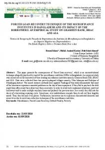
We investigate MDL model selection between the Poisson and geometric models. Figure 1 may help form an intuition about the probability mass functions of the two distributions. One reason for our choice of models is that they are both single parameter models, so that the n term of Equation 4 cancels. This means that at least for large sample sizes, dominant k2 ln 2π picking the model which best fits the data should always work. We nevertheless observe that for small sample sizes, data which are generated by the geometric distribution are misclassified as Poisson much more frequently than the other way around (see Section 5). So in an informal sense, even though the number of parameters is the same, the Poisson distribution is more prone to ‘overfitting’. To counteract the bias in favour of Poisson that is introduced if we just select the best fitting model, we would like to compute the third term of Equation 4, which now characterises the parametric complexity. But as it turns out, both models have an infinite parametric complexity; the integral in the third term of the approximation also diverges! So in this case it is not immediately clear how the bias should be removed. This is the second reason why we chose to study the Poisson and geometric models. In Section 4 we describe a number of methods that have been proposed in the literature as ways to deal with infinite parametric complexity; in Section 5 they are evaluated evaluate empirically. Reassuringly, all methods we investigate tend to ‘punish’ the Poisson model, and thus compensate for this overfitting phenomenon. However, the amount by which the Poisson model is punished depends on the method used, so that different methods give different results. We parameterise both the Poisson and the Geometric family of distributions by the mean µ ∈ (0, ∞), to allow for easy comparison. This is possible because for both models, the empirical mean (average) of the observed data is a sufficient statistic. For Poisson, parameterisation by 3

0.18 Poisson Geometric 0.16

0.14

0.12

0.1

0.08

0.06

0.04

0.02

0 0

5

10

15

20

Figure 1: The Poisson and geometric distributions for µ = 5. the mean is standard. For geometric, the reparameterisation can be arrived at by noting that in the standard parameterisation, P (x | θ) = (1 − θ)x θ, the mean is given by µ = (1 − θ)/θ. As a notational reminder the parameter is called µ henceforth. Conveniently, the ML estimator µ ˆ for both distributions is the average of the data (the proof is immediate if we set the derivative to zero). We will add a subscript p or g to indicate that codelengths are computed with respect to the Poisson model or the geometric model, respectively:

LP (xn | µ) = − ln n

LG (x | µ) = − ln

4

n Y e−µ µxi i=1

n Y i=1

xi !

=

n X i=1

µx i

(µ+1)xi +1

ln(xi !) + nµ − ln µ

= n ln(µ+1) − ln



n X

xi

(5)

i=1

µ µ+1

X n

xi

(6)

i=1

Four ways to deal with infinite parametric complexity

In this section we discuss four general ways to deal with the infinite parametric complexity of the Poisson and geometric models when the goal is to do model selection. Each of these four leads to one or sometimes more concrete selection criteria which we put into practice and evaluate in Section 5.

4.1

BIC/ML

One way to deal with the diverging term of the approximation is to just ignore it. The model selection criterion that results corresponds to only a very rough approximation of any real universal code, but it has been used and studied extensively. It was proposed both by Rissanen [15] and Schwarz [21] in 1978. Schwarz derived it as an approximation to the Bayesian marginal likelihood, and for this reason, it is best known as the BIC (Bayesian Information Criterion). Rissanen already abandoned the idea in the mid 1980’s in favour of more sophisticated approximations of the NML codelength.

4

k ln n 2 Comparing the BIC to the approximated NML codelength we find that in addition to the 1 term has also been dropped. This curious difference can be safely diverging term, a k2 ln 2π ignored in our setup, where k is equal to one for both models so the whole term cancels anyway. According to BIC, we must select the geometric model iff: LBIC (xn ) = L(xn | µ ˆ) +

0 < LP,BIC (xn ) − LG,BIC (xn ) = LP (xn | µ ˆ) − LG (xn | µ ˆ) We are left with a generalised likelihood ratio test (GLRT). Such a test has the form

PP(xn |θˆ) > η; PG(xn |θˆ)