Jun 29, 2005 - The paper presents empirical results which compare the robustness of two fitness functions used for software module clustering: one (MQ) used ...
An Empirical Study of the Robustness of Two Module Clustering Fitness Functions Mark Harman
Stephen Swift
Kiarash Mahdavi
King’s College Strand, London WC2R 2LS, UK.
Brunel University Uxbridge, Middlesex UB8 3PH, UK.
King’s College Strand, London WC2R 2LS, UK.
ABSTRACT Two of the attractions of search-based software engineering (SBSE) derive from the nature of the fitness functions used to guide the search. These have proved to be highly robust (for a variety of different search algorithms) and have yielded insight into the nature of the search space itself, shedding light upon the software engineering problem in hand. This paper aims to exploit these two benefits of SBSE in the context of search based module clustering. The paper presents empirical results which compare the robustness of two fitness functions used for software module clustering: one (MQ) used exclusively for module clustering. The other is EVM, a clustering fitness function previously applied to time series and gene expression data. The results show that both metrics are relatively robust in the presence of noise, with EVM being the more robust of the two. The results may also yield some interesting insights into the nature of software graphs.
Keywords Clustering, Modularization, Fitness Functions, Robustness
1.
INTRODUCTION
Search based module clustering has been used to automate the process of finding good choices of modularization for software systems which comprise many modules. The level of granularity of the clustering can be chosen to suit the application, so a module might denote (at the fine level of granularity) a single function or procedure or (at coarser levels of granularity) a file (which may contain many procedures and functions). Often, the modularization imposed when the system is first created becomes degraded as new modules are added to a system and as the existing modules are maintained. This degradation may be a signal, indicating the necessity for a phase of re-drawing the module boundaries as a part of the maintenance process. For some legacy systems, there is
Permission to make digital or hard copies of all or part of this work for personal or classroom use is granted without fee provided that copies are not made or distributed for profit or commercial advantage and that copies bear this notice and the full citation on the first page. To copy otherwise, to republish, to post on servers or to redistribute to lists, requires prior specific permission and/or a fee. GECCO’05, June 25–29, 2005, Washington, D.C., USA. Copyright 2005 ACM X-XXXXX-XX-X/XX/XX ...$5.00.
no ‘initial modularization’ available because the system was never created as a modular system. This makes maintenance much harder and migration to more, inherently modular, languages (such as object oriented styles) very time consuming and therefore costly [19]. In these situations, automation of the process of drawing module boundaries can be highly cost effective. Automated re-modularization through search based clustering analysis has been an area of much interest in search based software engineering, leading to the development of fast and effective tools for automated software module clustering. One of the attractions of search-based clustering (and of search–based software engineering itself [2]) arises from the robustness of the search algorithms. Software engineering problems are typically ‘messy’ problems in which the available information is often incomplete, sometimes vague and almost always subject to a high degree of change (including unforeseen change) [19]. In the case of modularization, the input information comes from dependence information collected from the source code of the program to be modularized. However, as programs evolve, their structure degrades, and so a legacy system may contain spurious dependencies which would be removed by restructuring. In other engineering fields, this characteristic of messiness, incompleteness and vagueness is typified by the presence of noise, and so the term ‘noise’ is used in this paper as an umbrella term to indicate the inherent uncertainty in the information available to an automated software module clustering system. The paper presents the results of an empirical study of the robustness of search based software module clustering using two fitness functions to guide the search: the MQ fitness function of Mancoridis et al. [13] and the EVM fitness function of Tucker et al. [22]. The representation of a software module clustering problem is expressed using a Module Dependency Graph, following Mancoridis et al. [13]. These may be referred to as MDGs or simply ‘graphs’ hereinafter. Data were collected for the application of search based clustering applied to six real and six artificial MDGs. The artificial systems allow a comparison of how the techniques behave when applied to perfect, real and random graphs. The experiments were repeated for mutated versions of the systems under study. The mutations of the systems represent the presence of increasing levels of noise in the data, facilitating a study of the robustness of the fitness functions as a guide to search based clustering algorithms.
extra–cluster relationships. Such a clustering achieves maximum possible cohesion and minimum possible coupling. The 1. Searches guided by both fitness functions degrade smoothly graphs with perfect clusterings were constructed to have a set of perfect clusters of nodes of increasing size. In all, the as noise increases, but EVM would appear to be the cluster sizes start with a single node, which, in the perfect more robust fitness function for real systems. clustering, belongs to a single module on its own, and range 2. Searches guided by MQ behave poorly for perfect and up to a cluster of size k, which, in the perfect clustering, is a near–perfect MDGs (though results degrade smoothly cluster of k nodes, all of which are related to each other and as noise is introduced, even for these graphs). no other nodes. Three perfect graphs were studied: The smallest with 55 nodes (with clusters of sizes: 1 to 10 in3. Tentatively, the difference in performance may shed clusive nodes), and the largest with 105 nodes (with cluster some light of the nature of program graphs themselves. sizes from 1 to 14 inclusive). These results must be treated with caution, but there is some evidence to suggest that program graphs are 2.2 Clustering Algorithm Used closer to perfect graphs (those for which an ideal modThe clustering algorithm used is based upon the Bunch ularization exists) than to arbitrary random graphs of algorithm [15]. This was re–implemented to create a tool equivalent edge density. BruBunch. The algorithm uses a hill climbing approach, like that in Bunch, but does not include the facility in Bunch to The rest of the paper is organised as follows: Section 2 remove omnipresent and library modules prior to clusterdescribes the experimental methods, subjects used, the two ing. An Omnipresent module is one which has many infitness functions studied and potential threats to validity. going and out–going relationships to other modules. Such Section 3 presents the results of the study and discusses modules would tend to belong in every cluster and so they the findings. Section 4 briefly describes related work and can adversely affect the results of clustering. Similarly, a Section 5 concludes. library module, is one which is used by a large number of modules (and which uses few itself). Library modules also tend to ‘belong’ in a large number of clusters. The Bunch 2. EXPERIMENTAL METHODS tool has facilities to remove these omnipresent and library This section describes the experimental methods used to modules so that their presence does not adversely affect the conduct the empirical study. Section 2.1 describes the subclustering search. ject programs and MDGs used. Sections 2.2 and 2.3 deThese two features were not included in BruBunch, howscribe the search algorithms and fitness functions used. Secever, because one of the goals of the experiment is to extions 2.4 and 2.5 describes the method used to model the plain the difference in behaviour for the clustering fitness effect of noise in the MDG and method used to assess clusfunctions, when applied to perfect, real and random graphs. tering similarity. Section 2.6 considers the threats to validity Perfect graphs contain many omnipresent modules (by defiof the results. nition), so these could not be removed while retaining comparability with results for other graphs. In all other re2.1 Subjects spects the BruBunch tool is a faithful re-implementation of An MDG is a graph in which nodes represent modules the Bunch tool, constructed according to the literature on and edges represent the dependence relationships between Bunch [15]. modules. Three types of MDG were studied: real program The BruBunch tool was created to allow experimentation MDGs, random MDGs and perfect MDGs. The real prowith different fitness functions for clustering and different gram MDGs come from six open source programs, ranging search strategies1 . in size from 20 modules to 174 modules, all of which are above the size for which search–space enumeration is possi2.3 Fitness Functions Used ble [15]. The details of these programs are summarised in Two fitness functions were experimented with: MQ, as Figure 1. Their MDGs were obtained using the programs’ implemented in Bunch and introduced by Mancoridis et al. files, where each file corresponds to a module. Where one [13], and the EVM function of Tucker et al. [22]. MQ has file uses another file, these uses are treated as module debeen used exclusively with Bunch and other work on softpendencies in constructing the Module Dependence Graphs. ware modularization [4, 12, 13, 14, 15, 16, 17]. EVM was The random graphs were obtained by constructing graphs introduced by Tucker et al. [22] and has been applied to with a random number of edges for three different numbers problems in time series data [22], and clustering of genes of nodes. The edge density (average number of outgoing according to gene expression data [7]. edges per node) was chosen to be identical to the average of The MQ function is inspired by software engineering conthat for the real programs studied (about 10% of the maxcerns of maximizing cohesion and minimizing coupling [3]. imum possible). Therefore, the random graphs are compaIt rewards clusterings for the presence of intra-module rerable with the real programs in size and edge density, but lationships and punishes them for the presence of extra– the connections are entirely random. Three random graphs 1 were studied, with different sizes: 50, 75 and 100 nodes Indeed, extensive experiments were carried out to attempt to find the best search strategy for clustering, including vari(modules). The details of these graphs are summarised in ations on hill climbing, genetic algorithms and simulated anFigure 1. nealing. None of these were found to outperform the Bunch A perfect graph, is so-named because it is one for which a algorithm in terms of the values of MQ for the clustering perfect modularization exists. That is, it is possible to clusfound by each search strategy. The results of these experiter the modules of the graph in such a way that all modules ments are beyond the scope of this paper, but they do sugin a cluster are related to all other modules and there are no gest that the Bunch algorithm is highly effective. The primary findings of this study are:
Name
# nodes
# edges
# EVM Evaluations
# MQ Evaluations
mtunis ispell rcs bison grappa incl
20 24 29 37 86 174
57 103 163 179 295 360
851,480 1,439,110 3,339,980 5,304,558 33,038,804 106,077,190
1,038,918 1,980,760 4,075,838 7,015,650 60,471,698 276,911,956
Perfect55 Perfect78 Perfect105
55 78 105
332 574 912
9,626,708 18,258,056 31,619,044
Random50 Random75 Random100
50 75 100
246 556 991
8,534,744 19,124,304 35,289,124
Description
Real Programs A simple operating system written in the Turing language A spelling checking utility A revision control system The GNU version of the yacc parser generator Evolutionary Algorithm tools A graph drawing tool Perfect MDGs 10,820,192 A set of completely connected sets of nodes of sizes 1 to 10 nodes 22,432,172 A set of completely connected sets of nodes of sizes 1 to 12 nodes 43,079,926 A set of completely connected sets of nodes of sizes 1 to 14 nodes Random MDGs 14,614,824 A 50 node random graph. Edge density = six real programs’ average 42,643,116 A 75 node random graph. Edge density = six real programs’ average 87,125,460 A 100 node random graph. Edge density = six real programs’ average
Figure 1: Subject programs studied module relationships. The EVM function was not defined with software engineering goals in mind. Nonetheless, it is similar, because it rewards clusterings which have a larger number of intra-module relationships. However, it does not directly punish clusterings which have extra–module relationships. Rather, for each cluster, c, it defines the score for the cluster in terms of the maximum possible set of intramodule relationships, incrementing the clusters’ score for each relationship which is present, and decrementing it for those which are absent. Therefore, it may indirectly punish high coupling, because a re–allocation of modules to clusters might turn high coupling between two modules into lower coupling between them and higher cohesion within one (possibly both) of them. In the following formal definitions of MQ and EVM, let a clustering C be defined to be a set of sequences {c1 , . . . , cm }, where each cluster ci is denoted by a sequence of elements, such that {c1 , . . . , cm } partitions C. Let ki be the size |ci | of the ith cluster of C. Let cij refer to the j th element of the ith cluster of C. The formal definition [22] of EV M (C) for clustering, C is
EV M (C) =
m X i=1
where, h(ci ), the score for cluster ci is defined as:
h(ci ) =
:
0
if ki > 1 otherwise
where L(cxy , cpq ) is defined as
L(cxy , cpq ) =
8 1 > >
> : −1
if there is a relationship from cxy to cpq or vice versa otherwise
The formal definition [15] of M Q(C) for a clustering, C is i=|C|
M Q(C) =
X i=1
CF(ci )
CF (ci ) = 2µi +
2µi Pj=|C|
j=1,j6=i
ǫij +ǫji
2
Where µi is the number of relationships between elements in cluster ci and ǫij is the number of relationships between elements of cluster ci and cluster cj . Strictly speaking, neither MQ nor EVM is a metric, since the value is not normalised. That is, in each case, the value of the function is the result of a summation over individual values for each cluster. Therefore, there are no upper bounds to the functions’ values. The EVM function has a global optimum corresponding to all modules in a single cluster, where the modules are all related to every other module. Similarly, for the ‘perfect’ MDGs, the perfect clustering corresponds to the global optimum for EVM. For MQ, the perfect clusterings do not correspond to global optima, as will be seen (see Section 3).
2.4 Modelling Noise
h(ci )
8 Pk −1 Pk i i < a=1 b=a+1 L(cia , cib )
Where the score, CF(ci ), awarded to a single cluster, ci is defined as follows:
In order to model the effect of noise, the MDGs studied are mutated by altering some of the edges of the graph. This mutation, allows the MDG to gradually differ from the original MDG from which it is created, with increases in difference created by larger amounts of mutation. The amount of mutation is measured as a percentage. A mutation of an MDG, m by x% represents the fact that x% of the entries in m’s adjacency matrix have been changed (either from 1 to 0 or 0 to 1). Put another way, for x% of the pairs of nodes in the graph denoted by m, an edge has been added or removed where one was absent or present (respectively). For each MDG studied, values of mutation from one to ten percent (in increments of one percent) were experimented with. As the mutation percentage increases, the MDG to which clustering algorithms are applied becomes less and less like the original and it is therefore expected that the similarity in the clustering produced (when compared to that of the original) will decrease. The interesting question is the way in which clustering similarity will decrease as the mutation rate increases.
2.5 Assessing Clustering Similarity and Collecting Results The Weighted–Kappa metric [1] was used to measure the similarity of two clusterings. The value of WK ranges from -1.0 to 1.0, with values in the range 0.2 to 0.6 representing weak agreement and values above 0.6 representing good agreement (with values above 0.8 representing very good agreement). The metric is computed in terms of a matrix of observations, with rows representing one observer and columns representing the other. In this case, the observers are clustering techniques. In general, there can be arbitrarily many observations, but in this case there are only two. That is, for a pair of nodes, the question is: ‘do these nodes occur in the same cluster or a different cluster?’. For each pair of nodes, a single observation is obtained. With two observers and two possible observations (same cluster, different cluster) there are four possible outcomes to a single paired observation. In two of these four outcomes, both observers agree (either agreeing on ‘same cluster’ or agreeing on ‘different cluster’). In the other two, they differ (one observes that the nodes are in the same cluster while the other observes that they are in different clusters). In general, where n observations are possible, an n–by–n matrix is constructed. In this case the matrix is a 2–by–2 matrix. The four elements of the matrix each denote the total number of occasions on which one of the four possible outcomes occur. On the leading diagonal, the two ‘agreement’ outcome totals are recorded: total number of pairs where both clusterings agree: ‘same cluster’ and total number of occasions where both clusterings agree: ‘different cluster’. The other two elements of the matrix record the two possible ‘disagreement’ outcomes. If the final value of the matrix contains zero in all places other than the leading diagonal, then the observers agree completely. In this case, it means that the clusterings are identical and the value of WK will be 1. If the clusterings are not identical, then some non-leading diagonal elements will be non-zero. At the extreme, where the leading diagonal consists solely of zero elements, then the clusterings are in complete disagreement about every pair of nodes and the value of WK will be -1. For the perfect graphs, the perfect clustering is known and so it is possible to compare the result of the clustering found by search with the perfect clustering. For all other graphs, the ‘perfect’ clustering is not known and so it is only possible to compare the clusterings produced for increasingly noisy versions of an MDG with the clustering obtained for the original MDG. In order to factor out the effects of randomness that are inherent in the application of hill climbing search techniques, the basic experiment was repeated ten times and the results reported are averages over these ten runs. Therefore, for each MDG, the WK metric is used to compare the results of the initial clustering obtained for the iteration of the experiment with each of those obtained for the subsequent ten runs of the increasingly mutated versions of the original MDG. In total, just over 280 million evaluations of the EVM fitness function were computed and 580 million evaluations of the MQ fitness function were computed. The number of evaluations of each fitness function, for each of the MDGs studied are reported in Figure 1.
2.6 Threats to Validity In any empirical study, it is necessary to consider the possible threats to the validity of the results. There were no human subjects in the empirical study reported here, and so threats to validity primarily fall into those of external and internal validity. The external validity concerns the extent to which it is possible to generalise from the results presented. In the case of the study reported here, the primary external threat to validity is the number and variety of programs considered. Are these typical? Can the results be considered to apply more widely? This is a common concern in empirical studies of software systems, because of the diverse nature of programs and the many differing applications to which they may be put. To address this concern, an attempt has been made to select a sample of programs with different application characteristics, including, tools, operating systems, utilities and application software and with sizes which vary by an order of magnitude. The threats to internal validity concern the possible selection bias in the choice of subjects and in the application of the experiment itself: Could the subjects could haver been chosen to show certain characteristics? Could the results could be a fluke, resulting from some random chance? The programs used in the study reported here were a subset of those used in other related studies [4, 13, 14, 15, 16, 17]. It is unlikely that there was any selection bias, since the experimenters could not have predicated the results from the MDGs due to the size of the search spaces involved. In order to mitigate concerns over the possibility that the results could have been obtained by random chance, the underlying experiment on robustness was repeated 10 times for each MDG and each fitness function and the results presented are the average over those 10 iterations.
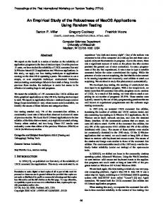
3. RESULTS AND ANALYSIS Figure 2 shows the results of the experiment for perfect MDGs described in Figure 1. Since these are graphs for which the perfect clustering is known, the Weighted–Kappa (WK) values are compared with those for the perfect clustering arrangement. In these figures, the horizontal axis shows the mutation percentage and the vertical axis shows the value of Weighted–Kappa. Each figure contains the results for both fitness functions for comparison, indicated by triangular points for MQ and square points for EVM. A point plotted at (x, y) indicates that, when the MDG is mutated by x percent, the average similarity (over 10 hill climbs) of the clustering produced when compared to the perfect clustering is y according to the Weighted–Kappa metric. In the three graphs depicted in Figure 2 a additional mutation percentage of 0% is included (this is not included in the results for non perfect MDGs which follow). This data point shows the level to which the set of 10 initial hill climbs agree with each other for the unmutated MDG. Figure 3 shows the results for the six real programs. The programs in Figures 3 are presented in order of increasing size (reading from top to bottom, then left to right). In the case of this and all other results (for non–perfect MDGs), the perfect clustering is not known. For these figures, a point plotted at (x, y) indicates that, when the MDG is mutated by x percent, the average similarity (over 10 hill climbs) of the clustering produced when compared to the cluster-
ing obtained for the unmutated MDG is y according to the Weighted–Kappa metric. To allow comparison with the results for the random and real MDGs, results were also collected to compare the clusterings of mutated versions of the perfect graphs with those obtained in the initial clustering (rather than compared with the perfect clustering). These results are depicted in Figure 4. Figure 5 shows the results of the experiment for the three random graphs described in Figure 1. In all these figures, the higher the values of WK achieved, the closer the agreement with the clustering obtained from the unmutated MDG (or the perfect clustering in the case of Figure 2). Clearly, the results for both fitness functions are better for perfect graphs than for random graphs (as expected). However, notice that the results for perfect graphs show that EVM produces clusterings which are perfect (for the perfect graph) and that the clusterings produced stay very close to the perfect results as more noise is introduced. This is true, both for the comparison against the perfect clustering (Figure 2), and the initial clustering (Figure 4). By comparison, the MQ fitness function performs much less well with these perfect MDGs. In Figure 4, both fitness functions are fairly robust (the Weighted–Kappa values remain relatively stable as the mutation rate increases). However, the similarity of the results of the MQ–guided searches with the initial clustering are much worse than those for the EVM-guided searches. Also, the initial set of 10 hill climbs all converge on the perfect clustering for EVM–guided searches, but not for the MQguided searches. Moreover, there is a ‘lack of agreement’ among the MQ–guided searches, not found in the EVM– guided searches. This behaviour can be explained by the nature of the MQ fitness function. It yields a value (between 0 and 1) for each cluster in a clustering. If a cluster has only relationships between members of the cluster and none to any elements outside the cluster, then the score for the cluster is 1 (the maximum possible). The value of MQ is the sum (over all clusters) for the score for each cluster. For a perfect MDG of n clusters, the reader might expect that MQ would have a value of n at its global optimum. However, this is not the case. The score obtainable using MQ for a perfect MDG of n clusters can be higher than n, because the clustering could contain more than n clusters, each of which does have a few relationships to modules outside the cluster, but each of which has a value only slightly lower than 1. Therefore, the global optimum of the MQ function does not correspond to the perfect clustering for a perfect MDG. Because of this, searches guided by MQ do not produce the perfect clustering for a perfect MDG, but a clustering with a higher MQ value. These results highlight a possible weakness in MQ as a guiding fitness function for modularization searches; it may be possible to improve upon it by addressing this issue. For random graphs, MQ and EVM degrade gracefully (there are no sharp drops in the graphs of Figure 5), but MQ produces clusterings which are consistently closer to the initial clustering, when compared to the results for EVM. That is, the graph of the degradation in MQ’s performance is always above that for EVM. This is interesting because it is precisely the reverse of the trend for perfect graphs. This observation is also interesting, when attention turns to the
graphs of real programs, depicted in Figure 3. For the real programs, EVM consistently produces clusterings which are closer to those for the initial MDG (with no noise) than the clusterings produced by MQ. These results must be treated with caution (see Section 2.6), but they do suggest some possible insights into the nature of software engineering graphs, when compared to graphs in general. The results show that EVM performs consistently better than MQ in the presence of noise for both perfect and real MDGs, but worse for random MDGs. The fact that these results appear to be so consistent for all six of the real programs indicates that there may be a trend here. It is tempting to speculate that the results of the experiments capture something of the nature of what constitutes a ‘real’ software engineering graph, rather than a purely random graph (or a ‘perfect’ graph). The results provides some empirical evidence for the claim that real systems have dependency graphs which ‘behave’ more like perfect graphs than they behave like random graphs. This would be perhaps a source of comfort to practitioners of software engineering; particularly those concerned with the maintenance of systems, where good modularization is so essential. It is also an interesting example of search based software engineering shedding potential insights into the nature of software engineering problems and artifacts, as well as providing a means to automate the search for good solutions. As the real programs in Figure 3 increase in size (as measured by number of nodes and edges in their MDGs), there appears to be a decrease in the difference between the performance of searches guided by EVM and those guided by MQ. With only six programs studied, any attempt at a statistical analysis of the significance of this apparent trend would be extremely questionable. However, the apparent trend is noteworthy: It may suggest that the choice of fitness function becomes less important as the size of a module increases; perhaps EVM is only more robust than MQ for smaller programs. Alternatively, it might suggest that, as system sizes increase, the graphs of systems’ dependence become more random in character and less like perfect graphs. Further study is required to provide a definitive answer. Overall, the results suggest that EVM may be worthy of further consideration as a means of assessing clustering quality. The results provide further evidence that search techniques are highly robust and degrade gracefully in the presence of noise in data (an optimistic finding for search based software engineering) and that the study of search based software engineering may be useful as a mechanism for shedding light on the nature of software engineering problems.
4. RELATED WORK The work reported here is most closely related to work on the Bunch tool, by Mancoridis, Mitchell et al. [4, 13, 14, 15, 16, 17], who introduced the search-based approach to software modularization in 1998 [14]. Harman et al. [5], studied the effect of assigning a particular modularization granularity as part of the search and Mahdavi et al. [11, 12] showed how multiple hill climbs could be used to identify building blocks which improve the behaviour of genetic algorithms when applied to the search–based modularization problems. However, despite many attempts in the litera-
mtunis
bison
ispell
grappa
rcs
incl
Figure 3: Results for the MDGs taken from Real Software Systems
ture [5, 12, 16], hill climbing has been found to be the most effective strategy for search–based clustering to date. A related problem of hierarchical decomposition of software is considered by Lutz [10]. Lutz is concerned with the problem of decomposition of software into hierarchies at different levels of abstraction, whereas the present work is concerned with only a single level of abstraction (the implementation level). Lutz therefore considers designs rather than code. More importantly, the fitness function used by Lutz, is based on an information-theoretic view point inspired by Shannon [21]. As such, it is very different from both MQ and EVM, so the results reported here do not have anything to say about such and information–theoretic approach to search–based modularization. Other authors have used the fitness functions themselves to assess properties of the software engineering problem under consideration. For example, Kirsopp et al. [8] use a sampling of the height of landscape peaks to assess aspects of the landscape for a feature subset selection problem applied to software cost estimation, while Pohlheim and Wegener [18] use exhaustive analysis of projections of the landscape to explore the characteristic of the landscape. The primary difference between these studies and that reported here lies
in the fact that the study here involved repeated hill climbs, rather than repeated fitness evaluations. Each hill climb involves many fitness evaluations, so the approach adopted here requires many more fitness evaluations to sample the search space. The results reported in Section 3 required over 860 million fitness function evaluations. Other work on software re-modularization has adopted analytical solutions based upon formal concept analysis and clustering fitness functions [6, 9, 23] and sets of heuristic rules [20].
5. CONCLUSIONS AND FUTURE WORK This paper has presented results concerning the robustness of two fitness functions EVM and MQ. Both fitness functions degrade smoothly as noise increases, but the EVM fitness function appears to be the more robust fitness function for real systems, suggesting that it may be worthy of further study as a guide for search–based module clustering. The results also compare performance of the two clustering fitness functions for perfect and entirely random graphs, suggesting some tantalizing (but highly tentative) observations about the nature of software systems. Specifically, the
Perfect55
Perfect55
Perfect78
Perfect78
Perfect105
Perfect105
Figure 2: Results for ‘Perfect’ MDGs Compared to the Perfect Clustering Result
Figure 4: Results for ‘Perfect’ MDGs Compared to generation zero
results appear to indicate that software systems are closer to ideal graphs, with perfect module clusterings, than they are to arbitrary random graphs of equivalent edge density. Future work will investigate these observations more deeply to explore the way in which search based software engineering can be used as a vehicle to improve understanding of the nature of software engineering problems.
Software Tools and Engineering Practice (STEP’99), Pittsburgh, PA, 30 August - 2 September 1999. M. Harman, R. Hierons, and M. Proctor. A new representation and crossover operator for search-based optimization of software modularization. In GECCO 2002: Proceedings of the Genetic and Evolutionary Computation Conference, pages 1351–1358, New York, 9-13 July 2002. Morgan Kaufmann Publishers. D. Hutchens and V. Basili. System structure analysis: clustering with data bindings. IEEE Transactions on Software Engineering, SE-11(8):749–757, 1985. P. Kellam, X. Liu, N. Martin, C. Orengo, S. Swift, and A. Tucker. A framework for modelling virus gene expression data. Intelligent Data Analysis, 6(3):267–279, 2002. C. Kirsopp, M. Shepperd, and J. Hart. Search heuristics, case-based reasoning and software project effort prediction. In GECCO 2002: Proceedings of the Genetic and Evolutionary Computation Conference, pages 1367–1374, New York, 9-13 July 2002. Morgan Kaufmann Publishers. C. Lindig and G. Snelting. Assessing modular
6.
REFERENCES
[1] D. G. Altman. Practical Statistics for Medical Research. Chapman and Hall, 1997. [2] J. Clark, J. J. Dolado, M. Harman, R. M. Hierons, B. Jones, M. Lumkin, B. Mitchell, S. Mancoridis, K. Rees, M. Roper, and M. Shepperd. Reformulating software engineering as a search problem. IEE Proceedings — Software, 150(3):161–175, 2003. [3] L. L. Constantine and E. Yourdon. Structured Design. Prentice Hall, 1979. [4] D. Doval, S. Mancoridis, and B. S. Mitchell. Automatic clustering of software systems using a genetic algorithm. In International Conference on
[5]
[6]
[7]
[8]
[9]
[14]
[15] Random50 [16]
[17]
Random75 [18]
[19] Random100 Figure 5: Results for MDGs of Random Graphs
[10]
[11]
[12]
[13]
structure of legacy code based on mathematical concept analysis. In Proceedings of the 1997 International Conference on Software Engineering, pages 349–359. ACM Press, 1997. R. Lutz. Evolving good hierarchical decompositions of complex systems. Journal of Systems Architecture, 47:613–634, 2001. K. Mahdavi, M. Harman, and R. Hierons. Finding building blocks for software clustering. In Genetic and Evolutionary Computation – GECCO-2003, volume 2724 of LNCS, pages 2513–2514, Chicago, 12-16 July 2003. Springer-Verlag. K. Mahdavi, M. Harman, and R. M. Hierons. A multiple hill climbing approach to software module clustering. In IEEE International Conference on Software Maintenance (ICSM 2003), pages 315–324, Amsterdam, Netherlands, Sept. 2003. IEEE Computer Society Press, Los Alamitos, California, USA. S. Mancoridis, B. S. Mitchell, Y.-F. Chen, and E. R. Gansner. Bunch: A clustering tool for the recovery and maintenance of software system structures. In Proceedings; IEEE International Conference on
[20]
[21]
[22]
[23]
Software Maintenance, pages 50–59. IEEE Computer Society Press, 1999. S. Mancoridis, B. S. Mitchell, C. Rorres, Y.-F. Chen, and E. R. Gansner. Using automatic clustering to produce high-level system organizations of source code. In International Workshop on Program Comprehension (IWPC’98), pages 45–53, Ischia, Italy, 1998. IEEE Computer Society Press, Los Alamitos, California, USA. B. S. Mitchell. A Heuristic Search Approach to Solving the Software Clustering Problem. PhD Thesis, Drexel University, Philadelphia, PA, Jan. 2002. B. S. Mitchell and S. Mancoridis. Using heuristic search techniques to extract design abstractions from source code. In GECCO 2002: Proceedings of the Genetic and Evolutionary Computation Conference, pages 1375–1382, New York, 9-13 July 2002. Morgan Kaufmann Publishers. B. S. Mitchell and S. Mancoridis. Using interconnection style rules to infer software architecture relations. In 8th Genetic and Evolutionary Computing Conference (GECCO’04), Seattle, USA, July 2004. Springer-Verlag. H. Pohlheim and J. Wegener. Testing the temporal behavior of real-time software modules using extended evolutionary algorithms. In W. Banzhaf, J. Daida, A. E. Eiben, M. H. Garzon, V. Honavar, M. Jakiela, and R. E. Smith, editors, Proceedings of the Genetic and Evolutionary Computation Conference, volume 2, page 1795, Orlando, Florida, USA, 13-17 July 1999. Morgan Kaufmann. R. Pressman. Software Engineering: A Practitioner’s Approach. McGraw-Hill Book Company Europe, Maidenhead, Berkshire, England, UK., 3rd edition, 1992. European adaptation (1994). Adapted by Darrel Ince. ISBN 0-07-707936-1. R. W. Schwanke. An intelligent tool for re-engineering software modularity. In Proceedings of the 13th International Conference on Software Engineering, pages 83–92, May 1991. C. E. Shannon. A mathematical theory of communication. Bell System Technical Journal, 27:379–423 and 623–656, July and October 1948. A. Tucker, S. Swift, and X. Liu. Grouping multivariate time series via correlation. IEEE Transactions on Systems, Man, and Cybernetics. Part B: Cybernetics, 31(2):235–245, 2001. A. van Deursen and T. Kuipers. Identifying objects using cluster and concept analysis. Technical Report SEN-R9814, Centrum voor Wiskunde en Informatica (CWI), Sept. 1998.