An Energetic Control Methodology for Exploiting the Passive Dynamics of Pneumatically Actuated Hopping Yong Zhu Eric J. Barth e-mail:
[email protected] Department of Mechanical Engineering, Vanderbilt University, Nashville, TN 37235
1
This paper presents an energetically derived control methodology to specify and regulate the oscillatory motion of a pneumatic hopping robot. An ideal lossless pneumatic actuation system with an inertia is shown to represent an oscillator with a stiffness, and hence frequency, related to the equilibrium pressures in the actuator. Following from an analysis of the conservative energy storage elements in the system, a control methodology is derived to sustain a specified frequency of oscillation in the presence of energy dissipation. The basic control strategy is to control the pressure in the upper chamber of the pneumatic cylinder to specify the contact time of the piston, while controlling the total conservative energy stored in the system to specify the flight time and corresponding flight height of the cylinder. The control strategy takes advantage of the natural passive dynamics of the upper chamber to provide much of the required actuation forces and natural stiffness, while the remaining forces needed to overcome the energy dissipation present in a nonideal system with losses are provided by a nonlinear control law for the charging and discharging of the lower chamber of the cylinder. Efficient hopping motion, relative to a traditional nonconservative actuator, is achieved by allowing the energy storing capability of a pneumatic actuator to store and return energy to the system at a controlled specifiable frequency. The control methodology is demonstrated through simulation and experimental results to provide accurate and repeatable hopping motion for pneumatically actuated robots in the presence of dissipative forces. 关DOI: 10.1115/1.2907355兴
Introduction
Pneumatic actuation presents a number of features not seen in typical robotic actuators. These features include a high mass specific power density relative to electromagnetic actuators, inherent compliance, and backdrivability, and the ability to controllably store and regenerate absorbed power. The combination of these three fairly distinct features makes pneumatic actuation an interesting candidate for untethered legged robots executing a cyclic gait. Hopping is studied here as a fundamental motion contained in many gaits. The goal of this work is to design a control methodology that results in energetically efficient oscillatory hopping motion when dissipation is present by taking advantage of the passive dynamics and energy storing capability of pneumatic actuation. Recent work 关1兴 on high energy-density monopropellant power supply and actuation systems for untethered robotics motivates an energetically savvy approach to the control of such systems with application to legged robots. Pneumatic actuation systems present the nearly unique opportunity among actuators to alter the physical stiffness, by varying the pressure, while still allowing an arbitrary force to be imposed, via the difference in pressures across the piston. Thus, the basic control strategy presented here is to control the physical stiffness of the actuation system to provide the majority of the required actuation forces passively and conservatively, while simultaneously controlling the total stored energy in the system to compensate for energy dissipation associated with contact, friction, leakage, and other losses. This is accomplished by controlling the pressure in one side of a pneumatic hopper to Contributed by the Dynamic Systems, Measurement, and Control Division of ASME for publication in the JOURNAL OF DYNAMIC SYSTEMS, MEASUREMENT, AND CONTROL. Manuscript received October 24, 2006; final manuscript received December 19, 2007; published online June 4, 2008. Assoc. Editor: George Chiu.
specify the contact time, while controlling the total stored system energy to specify the flight time and corresponding flight height. Suffering from highly nonlinear dynamics, varying environment conditions, and frequent phase transitions between free space and constrained motions, legged robot researchers generally face the challenge of free-space motion control, constrained motion control or force control, and issues of contact stability during the transition between the two. For an electrically actuated robot, if active force control is not implemented to effectively absorb the energy during contact, oscillations and even instability can occur. For example, joint acceleration feedback was used to control the contact transition of a three-link direct-drive robot 关2兴. Apart from active 共contact兲 force control, the passive compliance of tendons shows great advantages for the contact interaction tasks seen in legged locomotion. Inspired by nature, artificially engineered compliance such as series elastic actuators 关3兴 have been applied to walking robot applications as an alternative to direct force control. A hopping robot “Kenken” with an articulated leg and two hydraulic actuators as muscles and a tensile spring as a tendon was studied, although stability problems remained for higher speeds 关4兴. Aiming at both control and energetic efficiency, a monopod running robot with hip and leg compliance was controlled by taking advantage of the “passive dynamic” operation close to the desired motion without any actuation 关5兴. 95% hip actuation energy saving was shown at 3 m / s running speed. This idea is similar to the approach taken here, except here the compliance and hence passive dynamics will be specified by the compressibility of gas in a pneumatic actuator. In general, the natural compliance of pneumatic actuators has been proven to be of great importance when a robot interacts with an unknown passive environment 关6兴. In addition, the compliance of pneumatic actuators is a consequence of the compressibility of air and therefore represents a passive energy storage mechanism that provides an oppor-
Journal of Dynamic Systems, Measurement, and Control Copyright © 2008 by ASME
JULY 2008, Vol. 130 / 041004-1
Downloaded 13 Jun 2008 to 129.59.78.59. Redistribution subject to ASME license or copyright; see http://www.asme.org/terms/Terms_Use.cfm
tunity for enhancing the energy efficiency of pneumatically legged robots through controller design; the absorbed energy can be stored as the internal energy of compressed air and can be released again 共regeneration兲 in a controlled manner in another portion of the gait. Raibert was a pioneer in legged robot locomotion research using pneumatic cylinders. As an alternative to pneumatic cylinders, Mckibben actuators, or artificial muscles, have also been used for hopping robots to pursue higher power-to-weight ratios 关7兴. A dynamic walking biped “Lucy” actuated by pneumatic artificial muscles was investigated in Ref. 关8兴. Although artificial muscles can be used as actuators for legged robots and provide high power-to-weight ratios and shock absorption, they have many limitations and nonidealities such as hysteresis, short stroke, and undesirable nonlinear “end effects,” and will therefore not be considered further here. Raibert first presented the design and control of a pneumatic hopping robot in Ref. 关9兴. The hopping motion was generated in an intuitive manner. The upper chamber was charged when the foot is on the ground and exhausted as soon as it leaves the ground until it reached a predefined low pressure. There is a monotonic mapping between hopping height and thrust value, but this relationship cannot be simply characterized. The hopping height could only be chosen empirically. There is also a unique frequency associated with each thrust value, but this could only be implicitly regulated as well. Raibert used another leg actuation method for better efficiency 关9兴 when the hopping machine operated in three dimensions. The upper chamber worked as a spring and the lower chamber worked as an actuator. The upper chamber was connected to the supply pressure through a check valve. The lower chamber was charged when the foot is in flight and discharged when it was on the ground through a solenoid valve. By controlling the length of charging time during flight, the hopping height and frequency could be implicitly controlled. Although mentioned, energetic efficiency was not the main concern in Raibert’s work. In addition, the contact time and flight time could not be explicitly specified. Much research on legged robots using pneumatic systems was also carried out after Raibert. A small six-legged pneumatic walking robot named Boadicea was designed using customized lightweight pneumatic actuators and solenoid valves 关10兴. The performance clearly showed high force and power density over previous small scale robot designs. In other works similar to that presented here, fast gaits were generated for the control of a pneumatically actuated robot in Ref. 关11兴. The control system generated the desired trajectories in real-time and generated proper control inputs to achieve the desired trajectories. An energy-based Lyapunov function was chosen to generate the controlled limit cycles. This is similar to the approach taken here, except that this work will generate a desired velocity based on the current position and direction of motion. The contribution of the approach taken here over Raibert and others’ work is a control methodology built explicitly from the particular form of the conservative energy in such pneumatic systems. Contact stability is achieved inherently by the resulting closed-loop system being passive via regulation of the total stored conservative energy, and an interaction with an assumed passive environment. This paper therefore presents a control methodology that takes explicit advantage of the energy storage abilities and passive dynamics of pneumatic actuation applied to a hopping robot. The paper is organized as follows. In Sec. 2, it is shown that a lossless pneumatic actuation system is a natural oscillator that exchanges pneumatic potential energy and kinetic energy. Section 3 presents the specification of system parameters. Basically, desired hopping period and flight time are achieved through control of kinetic and potential energies of the system. Section 4 presents the control law to specify the desired kinetic and potential energies so that the desired hopping motion can be generated. Simulation results are shown in Sec. 5 where continuous control inputs 041004-2 / Vol. 130, JULY 2008
Fig. 1 Schematic diagrams of „a… a linear mass-spring system and „b… a vertical pneumatic system. An analysis of energetically lossless versions of both systems reveals equations of motion with an algebraic relationship between acceleration and position.
are provided by proportional valves. Section 6 presents experimental results of the pneumatic hopper where, instead of using proportional valves, solenoid on/off valves are used to carry out the same control approach. Conclusions are drawn in Sec. 7.
2
Energetic Analysis of a Pneumatic Oscillator
The conservative energy stored in a simple mass-spring linear oscillator not influenced by gravity 共Fig. 1共a兲兲 can be expressed as 1 1 E = 2 mx˙2 + 2 kx2
共1兲
For a system with no losses, taking the time rate of change of this expression and setting it equal to zero, E˙ = 共mx¨ + kx兲x˙ = 0
共2兲
yields not only the equation of motion of the system, but also reveals that the work rate, or power, injected into the system is always zero 共Fnetx˙ = 0兲. The resulting equation of motion necessary to keep the conservative energy constant, and the solutions x共t兲 = A sin共t兲, x˙共t兲 = A cos共t兲, x¨共t兲 = −A2 sin共t兲 = −2x共t兲, and = 冑k / m, both reveal a parameter dependent algebraic relationship between acceleration and position that specifies a frequency of sustained oscillation. A similar energetic analysis of the vertical pneumatic system shown in Fig. 1共b兲 also reveals an oscillatory system with a frequency of oscillation dependent upon system parameters. The kinetic and potential energy terms for a leakless, adiabatic 共no heat losses兲, frictionless piston-mass system while in contact with the ground are given as
共3兲 where Va,b represents the volume of chamber a or b, and Ar = Aa − Ab represents the cross sectional area of the piston rod. The potential energy of each chamber of the actuator is derived using standard thermodynamic relationships as the ability of the pressure in the chamber, Pa or Pb, to do work adiabatically with respect to an environment at atmospheric pressure Patm, where the ratio of specific heats is denoted by ␥. The term PEr共x兲 is a term similar to a gravitational potential energy term due to the unequal piston areas of the two sides of the actuator. If the system has no losses, the system will maintain a constant energy E by shuttling Transactions of the ASME
Downloaded 13 Jun 2008 to 129.59.78.59. Redistribution subject to ASME license or copyright; see http://www.asme.org/terms/Terms_Use.cfm
energy between potential and kinetic energy storages in the form of a well defined oscillation. Akin to the analysis for the simple mass-spring system subject to no energetic losses, the time rate of change of conservative energy storage is taken and set to zero as follows: E˙ = 关Mx¨ + PbAb − PaAa + PatmAr + Mg兴x˙ = 0
共4兲
Equation 共4兲 is obtained from Eq. 共3兲 by taking its time derivative and utilizing the fact that for a leakless, adiabatic system, the rate of change of internal energy storage is equal to the net rate of ˙ work done by side a or b, respectively 共U a,b
˙ ⇒ 共P˙ V + P V˙ 兲 / 共␥ − 1兲 = −P V˙ 兲. The = −W a,b a,b a,b a,b a,b a,b a,b equation of motion is evident from Eq. 共4兲 as follows:
correct 共5兲
Mx¨ = PaAa − PbAb − PatmAr − Mg
Substituting the following adiabatic relationships into the equation of motion, and defining static equilibrium pressures: Pa0 and Pb0 and volumes: Vmida and Vmidb at x = 0,
result in
␥ PaVa␥ = const = Pa0Vmida
共6兲
␥ PbVb␥ = const = Pb0Vmidb
共7兲
Pa0Aa − Pb0Ab − PatmAr − Mg = 0
共8兲
再 冋冉
Mx¨ + Pa0Aa
冊 冉 冊册 冊 册冎 冋 冉 ␥
Vmidb Vmidb − Abx
+ 共PatmAr + Mg兲 1 −
−
␥
Vmida Aax + Vmida
Vmidb Vmidb − Abx
␥
共9兲
=0
Fig. 2 Representative hopping trajectory
Pa0 =
共10兲
Vb = Vmidb − Abx
共11兲
PEa共x兲 =
FR = Pa0Aa
冋冉
冊 冉 冋 冉 ␥
Vmida − Aax + Vmida
Vmidb + 共PatmAr + Mg兲 1 − Vmidb − Abx
冊册
冏 冏 冋 冉 FR x
x=0
= ␥ Pa0Aa
PEb共x兲 =
冊册
共12兲
册 共13兲
This linear approximation and the following linearized equation of motion will be used in the subsequent development of specifying and controlling the hopping robot: Mx¨ + Kstiffx ⬵ 0
Vmida Vmida + Aax
Pa0 Vmida Patm Vmida + Aax
Pb0共Vmidb − Abx兲 1−␥
再冋 冉
冊冉
冊册
共14兲
It should also be noted that a rearrangement of Eq. 共13兲 gives the equilibrium pressure Pa0 in terms of a desired linear stiffness as follows: Journal of Dynamic Systems, Measurement, and Control
␥
␥ 共1−␥兲/␥
Vmidb Vmidb − Abx
Pb0 Vmidb Patm Vmidb − Abx
冊
冊册
−1
冊
冎
共16兲
␥
␥ 共1−␥兲/␥
−1
冎
共17兲 共18兲
Given that the stiffness of the pneumatic system increases as Pa0 and Pb0 increase, the frequency of oscillation is dependent upon these system parameters 共in addition to being amplitude dependent as determined by the total conservative energy stored in the system兲. Simple dynamic simulations of the system verify this claim.
3
冊
冉
再冋 冉
冊冉
PEr共x兲 = PatmArx
␥
Aa Ab Ab + − 共PatmAr + Mg兲 Vmida Vmidb Vmidb
Pa0共Vmida + Aax兲 1−␥
⫻
␥
Taking the partial derivative of FR evaluated at x = 0 gives the linearly approximated stiffness of the pneumatic actuator as follows: Kstiff =
冉
⫻
As seen in Eq. 共9兲, the pneumatic system shows a direct algebraic relationship between acceleration and position. Although nonlinear, the second term 共contained in brackets 兵 其兲 of Eq. 共9兲 plays a similar role as the position-dependent spring return force kx of the linear oscillator. We denote this return force as FR, Vmidb Vmidb − Abx
共15兲
A plot of the nonlinear stiffness due to the compressibility present in a pneumatic system shows that it has the effect of a hardening spring, given that the slope increases as x increases. Furthermore, it can also be seen that all potential energy terms in Eq. 共3兲 are a function solely of position, and therefore represent true pathindependent conservative energy potentials. Substitutions of Eqs. 共6兲 and 共7兲, in addition to Eqs. 共10兲 and 共11兲, result in expressions for the following position-dependent potentials:
where Va = Aax + Vmida
Kstiff/␥ + 共PatmAr + Mg兲Ab/Vmidb Aa共Aa/Vmida + Ab/Vmidb兲
Specification of System Parameters
This section will establish approximate relationships between the linearized stiffness and total conservative energy of the system, and the resulting time of flight and time on the ground of the hopping motion. This will provide a way to specify the two independent quantities of the system in terms of a desired dynamic behavior. 3.1 Defining the Hopping Cycle. For the system shown in Fig. 1共b兲 undergoing a representative hopping motion as shown in Fig. 2, the following critical moments and periods are defined: 共1兲 t0 = 0 defines the starting point of a full hopping cycle 共x = 0兲 共2兲 t1 defines the lift-up time of the foot 共y = 0兲 JULY 2008, Vol. 130 / 041004-3
Downloaded 13 Jun 2008 to 129.59.78.59. Redistribution subject to ASME license or copyright; see http://www.asme.org/terms/Terms_Use.cfm
共3兲 共4兲 共5兲 共6兲 共7兲
T1 = t1 − t0 is defined as the launch period T2 is defined as the compression period 共x 艋 0兲 Tair is defined as the flight time T3 is defined as the recovery period Thop is defined as the full hopping period
x共t1兲 ⬵
In the sections that follow, the hopping cycle will be analyzed according to the following decomposition: Thop ⬵ T1 + T3 + Tair + T2
共19兲
where Thop and Tair are to be specified, and T3 ⬵ T1. This relationship will then be utilized to determine the two independently specifiable quantities of desired stiffness, Kstiff, and desired total conservative energy Ed 共or alternatively Pa0 and Ed given that the relationship between Pa0 and Kstiff is a one-to-one mapping provided by Eq. 共15兲兲. Unfortunately, due to the coupling and nonlinearities present in the system, it is not possible to write closedform expressions for Kstiff and Ed in terms of Thop and Tair. Equation 共19兲 will therefore be cast as a function solely of the intermediate parameter T2 共the compression period兲 by pursuing the functional relationship T1共T2兲. Once the parameter T2 is determined, approximate closed-form expressions for Kstiff and Ed will be possible. This will allow a designer to specify Thop and Tair according to a desired gait, or other criteria, and arrive at initial values of system parameters Kstiff and Ed. These values can then be subsequently adjusted if further precision on Thop and Tair is required. 3.2 Launch Period T1. This section will express the launch period T1 as a function of the compression period T2. It should be first recognized that during the launch period, the system is in contact with the ground and approximately obeys the linear equation of motion Mx¨ ⬵ −Kstiffx given in Eq. 共14兲. The solution of this approximate equation of motion is x共t兲 ⬵ A sin共t兲
冉 冊
x共t1兲 ⬵ A sin
T1 T2
共21兲
The task is now to determine expressions for x共t1兲 and A as functions of the variable T2 and specifiable parameters Thop and Tair. To obtain an expression for x共t1兲 as a function of T2, consider the idealized lossless model of the hopping system as follows: Mx¨ = PaAa − PbAb − PatmAr − Mg
共22兲
my¨ = PbAb − PaAa + PatmAr + Fground − mg
共23兲
Utilizing Eq. 共23兲 with conditions immediately before contact is lost at time t1, namely, y˙ 共t1兲 = 0, ⌺Forces= 0 ⇒ y¨ 共t1兲 = 0, and Fground = 0, leads to the relationship PbAb − PaAa + PatmAr − mg = 0
共24兲
Substituting Eq. 共24兲 into Eq. 共22兲 with y˙ = 0 results in x¨共t1兲 = −
冉 冊
M+m g M
共25兲
which is the acceleration condition on x for the foot to break contact with the ground. Based on Eq. 共25兲, the approximate linear equation of motion Mx¨ = −Kstiffx given in Eq. 共14兲, and the fact that n,contact = 冑Kstiff / M = / T2 lead to the following:
冉 冊
Kstiff ⬵ T2
041004-4 / Vol. 130, JULY 2008
2
M
共26兲
共27兲
To obtain an expression for A in Eq. 共21兲 as a function of T2, consider the velocity x˙共t1兲 immediately before the foot breaks contact. Since both chambers are sealed when the foot is in the air, and by assuming the friction influence between the piston and cylinder wall is sufficient enough that relative motion between x and y can be neglected 共a mild assumption given most commercially available pneumatic cylinders兲, the time it takes for the cylinder body to reach the highest point is given by the simple free flight ballistics equation x˙共tpeak兲 = x˙共t1兲 − g共tpeak − t1兲
共28兲 1
Given that x˙共tpeak兲 = 0, and assuming that 共tpeak − t1兲 = 2 Tair, the launch velocity can be expressed in terms of Tair as follows: x˙共t1兲 =
Tairg 2
共29兲
1 1 Equating the kinetic energy at lift-off 2 共M + m兲x˙共t1兲2 = 8 共M 2 2 + m兲Tairg , with the potential energy at the peak 共M + m兲gh, with height h as the distance above the datum x共t1兲, results in the hopping height 1
共30兲
2 h = 8 gTair
The maximum position of the cylinder housing xmax can therefore be represented by combining Eq. 共30兲 with Eq. 共27兲 as follows: xmax = x共t1兲 + h =
共M + m兲g 1 2 + gT M共/T2兲2 8 air
共31兲
Although xmax is slightly higher than the absolute value of the minimum distance the cylinder housing can reach, it will be used as an approximation of the amplitude during contact as follows:
共20兲
Evaluated at the moment of lift-off, t1, and utilizing the fact that n,contact = 冑Kstiff / M = / T2 results in an expression that will provide the sought after relationship between T1 and T2,
共M + m兲g M共/T2兲2
A ⬵ xmax =
共M + m兲g 1 2 + gT M共/T2兲2 8 air
共32兲
Ideally, one would use the relationship A ⬵ 兩xmin兩 to more accurately approximate the amplitude of Eq. 共21兲, but unfortunately such an expression is not expressible as a function solely of the compression period T2 but instead depends upon both Kstiff and the total conservative energy E. It will be shown that the approximation of Eq. 共32兲 is acceptably accurate. Returning to Eq. 共21兲, and armed with expressions for x共t1兲 and A given by Eqs. 共27兲 and 共32兲, the launch period can be expressed as T1 ⬵
冉
8共M + m兲g T2 arcsin 2 8共M + m兲g + M共/T2兲2gTair
冊
共33兲
From both simulation and experimental results, it was seen that although the trajectory of x is quite symmetric, the trajectory of y is not as symmetric. To be able to specify the time the foot is in flight, it has been assumed that the y trajectory is symmetric about the highest point reached by x. However, since the foot generally bounces slightly when it lands on the ground, the time the foot is in the air cannot be easily determined. Due to this, the recovery period T3 is not strictly equal to the launch period T1, but equating these two quantities in Eq. 共19兲 will offer a reasonable approximation. 3.3 Solving for Kstiff and the Total Desired Conservative Energy. Utilizing Eq. 共33兲, Eq. 共19兲 can be expressed as Thop ⬵
冉
冊
8共M + m兲g 2T2 arcsin + Tair + T2 2 8共M + m兲g + M共/T2兲2gTair 共34兲
Equation 共34兲 is unfortunately a transcendental nonlinear equation that does not offer a closed-form solution for T2. Standard nonlinTransactions of the ASME
Downloaded 13 Jun 2008 to 129.59.78.59. Redistribution subject to ASME license or copyright; see http://www.asme.org/terms/Terms_Use.cfm
˙ ˙ ˙ = Pa,bVa,b + Pa,bVa,b U a,b ␥−1
共38兲
˙ =m ˙ a,bc pTflow H a,b
共39兲
˙ = P V˙ W a,b a,b a,b
共40兲
˙ = 0 共adiabatic兲: These result in the following for Q a,b
␥RTflow ␥ PaV˙a ˙a− P˙a = m Va Va
共41兲
␥RTflow ␥ PbV˙b ˙b− m P˙b = Vb Vb
共42兲
Taking the derivative of Eq. 共36兲 and substituting Eqs. 共41兲 and 共42兲 yield
តx =
冉
1 ␥ PbAbV˙b ␥ PaAaV˙a ␥RTflowAa ␥RTflowAb ˙a− ˙b − + m m M Vb Va Va Vb
冊
共43兲 Fig. 3 Schematic of a pneumatic hopping robot showing inertial coordinates for the cylinder housing „x… and piston „y… positions. „x = 0 at equilibrium pressures with y = 0 when the piston is in contact with the ground.…
ear solvers, such as MATLAB’s fzero routine, can be used to solve for T2 given known or specified values for M, m, Thop and Tair. Once the value of T2 has been determined, the sought after parameters Kstiff and Pa0 can be determined from Eqs. 共26兲 and 共15兲, respectively. The desired total conservative energy of the system to support the desired Thop and Tair can be obtained from the expression 1 Ed = 2 Mx˙共t1兲2 + PEa共x共t1兲兲 + PEb共x共t1兲兲 + PatmArx共t1兲 + Mgx共t1兲
共35兲 utilizing Eqs. 共29兲, 共27兲, 共16兲, and 共17兲 for quantities x˙共t1兲, x共t1兲, PEa共x共t1兲兲, and PEb共x共t1兲兲, respectively.
4
Controlled Pneumatic Hopping Robot
This section presents the system equations and control strategy for a vertical, gravity influenced pneumatic piston carrying an inertial load, serving as a hopping robot, as shown in Fig. 3. This system contains two exogenous control inputs in the form of control valves that influence the flow of mass into or out of each chamber a or b. The cylinder position and piston positions are defined as x and y, respectively, with separate origins as shown. By neglecting friction, leakage, and other losses, the dynamics of the vertical pneumatic cylinder housing 共while the system is in contact with the ground, or during flight兲 can be represented by the following equation: Mx¨ = PaAa − PbAb − PatmAr − Mg
共36兲
Expressions for the time rates of change of the pressures can be derived from the following constitutive relations for the rate of ˙ , rate of heat input Q ˙ , enthalpy rate H ˙, internal energy storage U ˙ , of each control volume associated with side a and work rate W and side b: ˙ =Q ˙ +H ˙ −W ˙ U a,b a,b a,b a,b
共37兲
Journal of Dynamic Systems, Measurement, and Control
˙ b, which can be ˙ a and m This system 共43兲 contains two inputs, m specified arbitrarily by the two control valves and an adequate supply pressure 关12–16兴. In practice, the pneumatic system shown in Fig. 3 will be subject to nonideal energetic losses including friction, leakage, heat losses, and losses due to impact with the ground when hopping. The aim of this work is to control the pneumatic system to oscillate and hop using the two control valves in order to inject energy to account for the energetic losses in the system. The control strategy will be to exploit the natural resonate dynamics of the pneumatic piston-mass system. Furthermore, it will be desirable to do so in a way to be able to specify and then regulate the time of flight and the total period of oscillation. One imaginable control approach would be to create a time dependent position trajectory from a simulation or analytical solution of the ideal lossless system, and then create a controller to have the controlled system follow this desired trajectory. This, however, would override the dynamics of the system with the expected dynamics and may not take full advantage of the natural passive dynamics of the system, depending on the degree of mismatch and the degree to which the control system would need to wrestle with the system. If taken advantage of, the passive dynamics can be utilized to help us achieve the task at hand in an energetically savvy manner by storing and returning energy among its conservative energy storage elements. Hence, the strategy taken here will be to regulate the stiffness of the system and the total amount of conservative energy stored in the system such that predictable and repeatable dynamic behavior is achieved in the face of dissipative losses. In brief, regulation of the stiffness of the system will be attained by using the control valve for chamber a 共see Fig. 3兲 in order to maintain the ideal position-dependent potential energy given by Eq. 共16兲. It should be reiterated that the equilibrium pressure Pa0 present in Eq. 共16兲 uniquely specifies the system’s stiffness 共as given in Eq. 共13兲兲. Maintenance of this stiffness will essentially scale time 共natural frequency兲 while in contact with the ground. The control valve for chamber b 共see Fig. 3兲 will be used to maintain the kinetic energy of the system. Due to the fact that all terms of Eq. 共3兲 except the kinetic energy are position dependent or a specified constant 共Ed兲, the desired velocity will be derived as a function of position. In this manner, the passive dynamics of the system will contribute constructively to a specified hopping motion. This strategy will be justified in the remainder of the paper. It should be noted that this strategy is based on the conservative energy storage expression of Eq. 共3兲, which is valid only while contact with the ground is maintained. In order to include the case JULY 2008, Vol. 130 / 041004-5
Downloaded 13 Jun 2008 to 129.59.78.59. Redistribution subject to ASME license or copyright; see http://www.asme.org/terms/Terms_Use.cfm
where ground contact is lost 共and regained, implying hopping兲, it will be sufficient to control the energy storage during contact only. The strategy is to therefore control the actuator only while it is in contact with the ground, and seal off the actuator while in flight 共both mass flow rates equal zero兲. Since it is known that the energy of the system when leaving and recontacting with the ground will be identical except for losses, controlling the energy profile while in contact will serve to compensate for the energy dissipation the system undergoes during both contact and flight. 4.1 Controlling the Potential Energy and Natural Frequency. The natural frequency of the pneumatic oscillator is specified via the dependence of the potential energy storage on position. It has been shown in Eq. 共16兲 that the scaling of this potential energy is dependent upon the equilibrium pressure Pa0. Therefore, utilizing Eq. 共6兲, the correct energy profile as a function of position is maintained if Pa is driven to the following desired pressure: Pad共x兲 = Pa0
冉
Vmida Vmida + Aax
冊
␥
共44兲
where Pa0 is determined from the desired periods Thop and Tair according to Sec. 3.3. Tracking this desired pressure as a function of position will compensate for leakage and heat losses and ensure that the correct amount of potential energy is stored in the system. In a manner akin to a spring, the correct amount of potential energy at each position will in turn ensure that the natural frequency of the passive dynamics contributes constructively to the desired hopping motion. To drive Pa to Pad, the following first order error dynamic with pole location −1 on the real axis is enforced during contact: e = Pa − Pad共x兲 = Pa − Pa0
冉
Vmida Vmida + Aax
冊
␥
共45兲
e˙ + 1e = 0
共46兲
P˙a − P˙ad共x兲 = − 1共Pa − Pad共x兲兲
共47兲
Substituting in Eq. 共41兲 for P˙a, and its idealized form for P˙ad共x兲, P˙ad共x兲 = −
␥ PaAax˙ 共Vmida + Aax兲
共48兲
冉
1共Vmida + Aax兲 Aax˙ + ␥RTflow RTflow
冊冉
Pa − Pa0
冉
Vmida Vmida + Aax
冊冊
⫻sgn
where Tflow is approximated to be room temperature. 4.2 Controlling the Kinetic Energy. Merely maintaining the proper potential energy profile as a function of position is not sufficient to sustain a cyclic motion in the face of dissipation. By additionally ensuring the correct amount of kinetic energy as a function of position, a well regulated cyclic motion while in contact with the ground can be achieved. During flight, and as evidenced by Eq. 共29兲, the flight time is dependent upon the launch velocity at the critical lift-off position x共t1兲. Therefore, in controlling the hopping robot subject to losses, it will be critical to maintain the correct velocity at each position during contact. The total desired conservative energy of the system, Ed, in terms of the desired periods Thop and Tair is specified in Sec. 3.3. By utilizing this quantity for E in Eq. 共3兲, the following positiondependent desired velocity can be defined to maintain the desired conservative energy while in contact:
2 共Ed − PEa共x兲 − PEb共x兲 − PEr共x兲 − Mgx兲 M
2 共Ed − PEa共x兲 − PEb共x兲 − PEr共x兲 − Mgx兲 M
冊
冏
共50兲
where PEa共x兲, PEb共x兲, and PEr共x兲 are evaluated according to Eqs. 共16兲–共18兲, respectively, with the value of Pb0 evaluated according to Eq. 共8兲. The resulting shape of the desired position-dependent velocity profile according to Eq. 共50兲 is shown in Fig. 4. Note that this position-based desired velocity also depends on the sign of the current velocity. Based on Eq. 共9兲, the desired acceleration can also be expressed as a function of position, x¨d共x兲 =
再 冋冉
1 Pa0Aa M
冊 冉 冊册 冊 册冎 冋冉
Vmida Aax + Vmida
+ 共PatmAr + Mg兲
␥
−
Vmidb Vmidb − Abx
Vmidb Vmidb − Abx
␥
−1
␥
共51兲
As will be seen, the desired jerk is required as a feedforward term in the control law as follows:
冋
␥ ␥A2a Pa0Vmida 1 − M 共Vmida + Aax兲1+␥
␥
共49兲
041004-6 / Vol. 130, JULY 2008
冑冏 冉
x˙d共x兲 = sgn共x˙兲
តxd共x,x˙d兲 =
results in the following control law for chamber a: ˙a= − m
Fig. 4 Representative position-dependent velocity profile
−
册
␥ ␥Ab共Pa0Aa − PatmAr − Mg兲Vmidb x˙d 1+␥ 共Vmidb − Abx兲
共52兲
The desired position-dependent acceleration profile is shown in Fig. 5. It should also be noted that the relationship between acceleration and position revealed by Eq. 共51兲, and shown in Fig. 5 below, is very nearly linear for a large range of positions 共80% of the total stroke of the actuator兲. This large linear range substantiates the use of the approximate equation of motion Mx¨ + Kstiffx ⬵ 0 given in Eq. 共14兲 and the linear stiffness term given in Eq. 共13兲. The desired velocity can be achieved through a simple nonlinear control law to track the desired position-dependent velocity through valve b. The Lyapunov-based control law derivation can be summarized as follows: 1
V = 2 s2
共53兲
s = 共x¨ − x¨d兲 + 2共x˙ − x˙d兲
共54兲
V˙ = ss˙ = − k2s2
共55兲
Transactions of the ASME
Downloaded 13 Jun 2008 to 129.59.78.59. Redistribution subject to ASME license or copyright; see http://www.asme.org/terms/Terms_Use.cfm
Fig. 5 Representative position-dependent acceleration profile
s˙ = − k2s
共56兲
s˙ = 共xត − ត xd兲 + 2共x¨ − x¨d兲 = − k2s
共57兲
Fig. 6 Hopping results for designed periods of Thop = 0.4 s and Tair = 0.2 s. Actual periods in simulation are Thop = 0.39 s and Tair = 0.18 s.
Fground = − kgroundy − bgroundy˙
if y ⬍ 0
共62兲
where kground = 1.0⫻ 10 N / m and bground = 1000 N s / m. The control laws for each side of the piston are given by Eqs. 共49兲 and 共59兲, respectively, with 1 = 1000, 2 = 400, and k2 = 40, during ˙ b = 0 during flight 共y ⬎ 0兲. ˙ a=m contact 共y 艋 0兲; and m Figures 6 and 7 show simulations results of the hopper for designed periods of Thop = 0.4 s and Tair = 0.2 s. Hopping is present as evidenced by the piston position y becoming nonzero in Fig. 6. It can be seen that the approximations of Sec. 3.3 provided parameters Pa0 and Ed that result in reasonably close approximations of the desired periods Thop and Tair. Figure 7 shows the controlled mass flow rates, demonstrating that the hopper achieves the designed behavior largely through its passive dynamics. 6
តx = តxd − 2共x¨ − x¨d兲 − k2s
共58兲
where 2 and k2 specify the dynamics on and off the sliding sur˙a face, respectively. Substitution of Eq. 共43兲 into Eq. 共58兲 with m = 0 yields the control law for side b as follows: ˙b=− m
冋 册
␥ PaV˙aAa ␥ PbV˙bAb MVb − +ត xd − 共2 + k2兲共x¨ − x¨d兲 ␥RTflowAb MVa MVb
− k22共x˙ − x˙d兲
共59兲
where Tflow is again approximated to be room temperature. Achieving the control mass flow rates specified in Eqs. 共49兲 and 共59兲 can be done with two three-way valves 共one per side a and b兲 to charge or discharge the piston chambers. In the case of proportional valves that modulate the flow orifice area, there is a direct algebraic relationship between orifice area and mass flow rate 关12–16兴. This relationship can be utilized to command the valve orifice area. For a sufficiently high bandwidth valve, the dynamics associated with achieving the needed orifice can be, and is commonly, neglected.
6
Experimental Implementation Using Solenoid Valves
To implement the proposed hopping control, the use of proportional valves presents a costly and bulky option for a system that is ideally lean and inexpensive. If the proposed hopping control is to be part of a multilegged robot where the vertical frequency of gait at each limb is addressed with the proposed methodology, the
5 Hopping Simulation Results Using Proportional Valves A simulation of a controlled pneumatic hopping robot involving frictional losses is presented below. The hopping system was modeled as follows: Mx¨ = PaAa − PbAb − PatmAr − Mg − b共x˙ − y˙ 兲
共60兲
my¨ = PbAb − PaAa + PatmAr + Fground − mg − b共y˙ − x˙兲
共61兲
with M = 0.54 kg and m = 0.05 kg, and viscous friction effects representing the sliding piston and rod seals modeled by b = 2 N s / m. The supply pressure, utilized in the mass flow relationships 关12兴, was set as 652.2 kPa 共80 psi 共gauge兲兲. The mass parameters and supply pressure are the same as the experimental setup, which will be described in Sec. 6. The pressure dynamics were modeled as Eqs. 共41兲 and 共42兲. The ground model was approximated as a very stiff spring and damping to represent losses upon collision, Journal of Dynamic Systems, Measurement, and Control
˙ a and m ˙a Fig. 7 Control mass flow rates m
JULY 2008, Vol. 130 / 041004-7
Downloaded 13 Jun 2008 to 129.59.78.59. Redistribution subject to ASME license or copyright; see http://www.asme.org/terms/Terms_Use.cfm
number of valves needed quickly becomes prohibitive in terms of both cost and size. More importantly, proportional spool valves are not necessary to implement the proposed control methodology given that the method takes advantage of the passive dynamics of the system for the majority of the control task and only utilizes mass flow to maintain the correct passive dynamics. As seen in Fig. 7, the required mass flow comes only in short shots. Therefore, to make future pneumatic powered walking machines more feasible, while exploiting the energetic approach of the proposed controller, simple on/off three-way solenoid valves are used in the experiments. To carry out the proposed control approach with on/off threeway valves, some modification of the control laws 共49兲 and 共59兲 is required. As an alternative to the control of side a, consider the error signal of Eq. 共45兲. Instead of specifying a particular error dynamic as done in Eq. 共46兲, consider instead the following positive definite Lyapunov function: 1
共63兲
V = 2 e2 At the simplest level, it is desired to ensure the following: V˙ = ee˙ = 共Pa − Pad兲共P˙a − P˙ad兲 艋 0
while e ⫽ 0
冉 冊
while 共Pa − Pad兲 ⬍ 0
V˙ 苸 兵V˙ Ps,V˙ PbV˙ Patm其
Charge chamber a if Pa ⬍ Pa0
冉
冊
␥
if 共V˙ Pb 艋 0兲 then ub = Pb else if 共V˙ Ps 艋 0兲 then ub = Ps else if 共V˙ Patm 艋 0兲 then ub = Patm else
共65兲
ub = input associated with min共V˙兲
and y 艋 0
To control side b using an on/off valve, the on/off control methodology of Ref. 关17兴 will be used. The derivation of this control law is summarized briefly here. With v and s defined as before in Eqs. 共53兲 and 共54兲, s˙ can still be represented as
ត − តxd兲 + 2共x¨ − x¨d兲 s˙ = 共x
共67兲
It will be necessary to enforce the following condition: xd兲 + 2共x¨ − x¨d兲兴 艋 0 V˙ = ss˙ = 关共x¨ − x¨d兲 + 2共x˙ − x˙d兲兴关共xត − ត 共68兲 Taking the derivative of Eq. 共36兲 gives 共69兲
˙ a = 0 and a linearized form of the Substitution of Eq. 共41兲 with m pressure dynamics P˙b = 共ub − Pb兲 / b 关17兴 yields
ត= − Mx
ub − Pb ␥ PaV˙a Aa − Ab Va b
共70兲
where b is a time constant determined by pressure response. In accordance to the three positions of the valves 共charge, seal, or discharge兲 the input term of Eq. 共70兲 is only a finite set of discrete values, 041004-8 / Vol. 130, JULY 2008
end if end if end if
共66兲
Mxត = P˙aAa − P˙bAb
共72兲
To track the desired position based velocity trajectory by enforcing Eq. 共68兲 and utilize the least amount of compressed air from the supply, the following switching control law is implemented while in contact with the ground:
Since Eq. 共65兲 simply states that the mass flow rate must be greater than some number when the chamber is under pressurized, the following on/off control law will be used for side a while in contact with the ground: Vmida Vmida + Aax
共71兲
Substitution of Eq. 共70兲 into Eq. 共68兲 yields a candidate V˙ associated with each input value. Each V˙ candidate can be computed online in real time.
共64兲
Furthermore, as stated previously, the control of side a compensates mostly for leakage and it is realistically only required to occasionally pressurize the chamber. This corresponds to the actual pressure being lower than the desired pressure 共Pa − Pad兲 ⬍ 0. Upon substitution of Eqs. 共41兲 and 共48兲 for the case of 共Pa − Pad兲 ⬍ 0, the following condition arises: Aax˙ ˙ a 艌 共Pa − Pad兲 m RTflow
ub 苸 兵Ps, Pb, Patm其
That is, sealing off the chamber, which is the first priority if this option, presents a negative definite candidate V˙ Pb 艋 0. If this candidate is not negative definite, then charging the chamber is the second consideration for velocity tracking convergence. If both of these control options cannot make the velocity tracking converge, then discharge is used. If none of these can enforce a negative definite V˙, which means that V˙ ⬎ 0 for any of the three possible inputs, the one associated with the minimum V˙ is chosen as the input. This slight violation of Eq. 共68兲 is discussed in Ref. 关17兴. The experimental setup is shown in Fig. 8. The pneumatic actuator is a long, small diameter double acting cylinder 共Bimba 0078-DXP兲 with a stroke length of 10 in. 共254 mm兲, piston diameter of 0.39 in. 共9.91 mm兲, and piston rod diameter of 1 / 8 in. 共3.175 mm兲. A linear potentiometer 共Midori LP-150F兲 with 150 mm maximum travel is used to measure the vertical position of the cylinder housing, and a linear potentiometer 共Midori LP100F兲 with 100 mm maximum travel is used to measure the vertical position of the piston. The velocity of the cylinder was obtained from position by utilizing a differentiating filter with a 20 dB/ decade roll-off at 100 Hz. The acceleration signal was obtained from the velocity signal with a differentiating filter with a 20 dB/ decade roll-off at 30 Hz. Given the range of desired frequencies of operation, these differentiating filters added negligible phase lag. Two pressure transducers 共Festo SDE-16-10V/20mA兲 are attached to each cylinder chamber, respectively. Control is provided by a Pentium 4 computer with an analog-to-digital 共A/D兲 card 共National Instruments PCI-6031E兲, which controls the two solenoid valves through two digital output channels. The moving mass is about 0.54 kg. Two two-way, three-position 共charge, disTransactions of the ASME
Downloaded 13 Jun 2008 to 129.59.78.59. Redistribution subject to ASME license or copyright; see http://www.asme.org/terms/Terms_Use.cfm
Fig. 8 Photograph of the experimental setup
Fig. 11 Case III: hopping results for designed periods of Thop = 0.45 s and Tair = 0.15 s. Actual experimental periods „consistent after the fourth hop… are Thop = 0.44 s and Tair = 0.17 s.
Fig. 9 Case I: hopping results for designed periods of Thop = 0.35 s and Tair = 0.1 s. Actual experimental periods are Thop = 0.36 s and Tair = 0.14 s.
Fig. 10 Case II: hopping results for designed periods of Thop = 0.4 s and Tair = 0.2 s. Actual experimental periods are Thop = 0.46 s and Tair = 0.18 s.
Journal of Dynamic Systems, Measurement, and Control
charge, sealed兲 solenoid valves 共Numatics MircroAir series M10SS641M000061兲 are attached to the chambers. The valve manufacturer reports a valve opening and closing time of 14 ms and 18 ms, respectively. This response time is at least two orders of magnitude faster than the range of hopping periods for the system with the selected components above, and should therefore not present any appreciable effects related to time delay. The supply pressure was set as 652.2 kPa 共80 psi 共gauge兲兲, the same as the simulation cases. Three sets of experimental results are included in Figs. 9–14 below to show that the hopping frequency can be explicitly controlled and hopping height can be implicitly regulated. These three cases are the following. Case I: designed periods of Thop = 0.35 s and Tair = 0.1 s. Case II: designed periods of Thop = 0.4 s and Tair = 0.2 s. Case III: designed periods of Thop = 0.45 and Tair = 0.15 s. Table 1 shows a summary of the experimental results for the three cases. Figures 9–11, show the position response of the system for each case. Figure 12 shows the velocity tracking for Case II where, again, this is only achieved or expected during contact. Figure 13 shows the pressure tracking in chamber a for Case II
Fig. 12 Case II: desired velocity „x˙d… and actual velocity „x˙…. Velocity tracking is achieved during contact only.
JULY 2008, Vol. 130 / 041004-9
Downloaded 13 Jun 2008 to 129.59.78.59. Redistribution subject to ASME license or copyright; see http://www.asme.org/terms/Terms_Use.cfm
Fig. 13 Case II: desired pressure „Pad… and actual pressure „Pa… in chamber a. Pressure tracking is achieved during contact only.
Fig. 14 Case II: discrete valve control signals
Table 1 Summary of experimental results
Case I Case II Case III
Thop desired 共s兲
Thop actual 共s兲
Tair desired 共s兲
0.35 0.40 0.45
0.36 0.46 0.44
0.10 0.20 0.15
where this is only achieved during contact. Figure 14 shows the discrete valve control signals during Case II. Comparing the experimental result shown in Fig. 10 with the simulation result shown in Fig. 7 for the same desired Thop = 0.4 s and Tair = 0.2 s, it can be seen that the solenoid valves provide very similar experimental results that match the simulation results well in terms of hopping height 共x and y兲 and time periods 共Thop and Tair兲. Although the velocity tracking shown in Fig. 12 is not very accurate, the total conservative energy is still compensated during contact; this is verified by the consistent hopping height shown in the position trajectories. Finally, it should be noted that the maximum stiffness was limited in experiment by the supply pressure coupled with leakage. The minimum stiffness was limited by physical constraints of the setup, as can be seen in the first compression of Case III “bottoming out” in Fig. 11.
7
Conclusions
This paper presents the design of a “natural” pneumatic hopping robot that exploits the passive dynamics of the system to achieve a desired period of oscillation and a desired time of flight. By allowing the passive dynamics of the system to provide the majority of the desired dynamics, the energy storing capability of a pneumatic actuator is exploited. This results in a more energetically efficient hopping motion relative to the alternative of providing all of the required forces via a nonconservative actuation scheme. The energetic approach also allows for inherent contact stability to be achieved. Regulation of the conservative energy of the system results in an overall passive closed-loop system, which inherently interacts in a stable manner with a passive environment. To achieve the actual passive dynamics of the system, as opposed to the estimated passive dynamics, the control approach is position based. This position-based control approach effectively specifies desired trajectories as a function of position as opposed to the more typically utilized time-based desired trajectories. The 041004-10 / Vol. 130, JULY 2008
Tair actual 共s兲
Kstiff desired 共N/m兲
Ed desired 共J兲
Pa0 desired 共kPa兲
192.6 204.4 122.1
10.29 11.44 5.03
468.2 493.1 319.3
0.14 0.18 0.17
desired pressure as a function of position is generated for one chamber of the actuator and tracked to regulate the natural frequency of the pneumatic cylinder. Desired velocity, acceleration, and jerk are scheduled as functions of position and then tracked using the pressure of the rod side of the actuator to regulate the kinetic energy of the system and hence hopping amplitude and flight time. The analysis showed that the position-dependent desired behavior ensures that the passive dynamics of the system are energetically exploited to achieve the desired motion. Essentially, a position-dependent control approach ensures that the passive natural frequencies of the system are achieved without requiring a high accuracy model of the process, load, or disturbances. This is in contrast to utilizing the parameters of the system to estimate the natural frequency, specifying a time-based behavior, and then needing to fight the natural dynamics to match the difference between the estimated and actual natural frequency of the system. The resulting control is activated only during contact. During flight, the energy of the system is stored and returned as additional gravitational energy. Additionally, given that the control methodology is position based, variations in flight time or disturbances during flight will not affect the degree to which the passive dynamics are beneficially exploited. Finally, the control laws for proportional valves were modified for the use of simple solenoid on/off valves. Simulation and experimental results demonstrated the accuracy and consistency of the proposed control methodology.
References 关1兴 Goldfarb, M., Barth, E. J., Gogola, M. A., and Wehrmeyer, J. A., 2003, “Design and Energetic Characterization of a Liquid-Propellant-Powered Actuator for Self-Powered Robots,” IEEE/ASME Trans. Mechatron. 8 共2兲, pp. 254– 262. 关2兴 Xu, W. L., Han, J. D., and Tso, S. K., 2000, “Experimental Study of Contact Transition Control Incorporating Joint Acceleration Feedback,” IEEE/ASME Trans. Mechatron. 5共5兲, pp. 292–301.
Transactions of the ASME
Downloaded 13 Jun 2008 to 129.59.78.59. Redistribution subject to ASME license or copyright; see http://www.asme.org/terms/Terms_Use.cfm
关3兴 Williamson, M. M., 1995, “Series Elastic Actuators,” Ms thesis, MIT, Cambridge, MA. 关4兴 Hyon, S. H., and Mita, T., 2002, “Development of a Biologically Inspired Hopping Robot—‘Kenken’,” Proceedings of the 2002 IEEE International Conference on Robotics & Automation, Washington, DC, pp. 3984–3991. 关5兴 Hmadi, M., and Buehler, M., 1997, “Stable Control of a Simulated One-legged Running Robot With Hip and Leg Compliance,” IEEE Trans. Rob. Autom., 13共1兲, pp. 96–104. 关6兴 Guihard, M., and Gorce, P., 2004, “Dynamic Control of a Large Scale of Pneumatic Multichain Systems,” J. Rob. Syst., 21共4兲, pp. 183–192. 关7兴 Delson, N., Hanak, T., Loewke, K., and Miller, D. N., 2005, “Modeling and Implementation of McKibben Actuators for a Hopping Robot,” Proceedings of the 12th Annual International Conference on Advanced Robotics 共ICAR兲, Seattle, WA, pp. 833–840. 关8兴 Verrelst, B., 2005, “A Dynamic Walking Biped Actuated by Pleated Pneumatic Artificial Muscles: Basic Concepts and Control Issues,” Ph.D dissertation, Vrije Universiteit Brussel, Brussels, Belgium. 关9兴 Raibert, M., 1986, Legged Robots That Balance, MIT, Cambridge, MA. 关10兴 Binnard, M. B., 1995, “Design of a Small Pneumatic Walking Robot,” Ms thesis, MIT, Cambridge, MA. 关11兴 M’sirdi, N. K., Manamani, N., and Nadjar-Gauthier, N., 1998, “Methodology Based on CLC for Control of Fast Legged Robots,” Proceedings of the 1998
Journal of Dynamic Systems, Measurement, and Control
关12兴 关13兴 关14兴 关15兴 关16兴 关17兴
IEEE/RSJ International Conference on Intelligent Robotics and Systems, Victoria, B. C., Canada, pp. 71–76. Richer, E., and Hurmuzlu, Y., 2000, “A High Performance Pneumatic Force Actuator System: Part I—Nonlinear Mathematical Model,” ASME J. Dyn. Syst., Meas., Control, 122共3兲, pp. 416–425. Richer, E., and Hurmuzlu, Y., 2000, “A High Performance Pneumatic Force Actuator System: Part II—Nonlinear Control Design,” ASME J. Dyn. Syst., Meas., Control, 122共3兲, pp. 426–434. Zhu, Y., and Barth, E. J., 2005, “Impedance Control of a Pneumatic Actuator for Contact Tasks,” in Proceedings of the 2005 IEEE International Conference on Robotics and Automation, pp. 999–1004. Al-Dakkan, K., Goldfarb, M., and Barth, E. J., 2003, “Energy Saving Control for Pneumatic Servo Systems,” Proceedings of the 2003 IEEE/ASME International Conference on Advanced Intelligent Mechatronics, pp. 284–289. Fite, K. B., and Goldfarb, M., 2006, “Design and Energetic Characterization of a Proportional-injector Monopropellant-Powered Actuator,” IEEE/ASME Trans. Mechatron. 11共2兲, pp. 196–204. Barth, E. J., and Goldfarb, M. 2002, “A Control Design Method for Switching Systems with Application to Pneumatic Servo System,” 2002 ASME International Mechanical Engineering Congress & Exposition, New Orleans, LA, Nov.
JULY 2008, Vol. 130 / 041004-11
Downloaded 13 Jun 2008 to 129.59.78.59. Redistribution subject to ASME license or copyright; see http://www.asme.org/terms/Terms_Use.cfm