an energy-efficient distributed schedule- based ...

‫‪T. A. Al-Khdour and U. Baroudi‬‬

‫‪AN ENERGY-EFFICIENT DISTRIBUTED SCHEDULE‬‬‫‪BASED COMMUNICATION PROTOCOL FOR PERIODIC‬‬ ‫‪WIRELESS SENSOR NETWORKS‬‬ ‫*‪T. A. Al-Khdour‬‬ ‫‪COE Dept., KFUPM, P.O Box 8545, Dhahran 31261, Saudi Arabia‬‬

‫‪and U. Baroudi‬‬ ‫‪COE Dept., KFUPM, P.O Box 5065, Dhahran 31261, Saudi Arabia‬‬

‫اﻟﺨﻼﺻـﺔ‪:‬‬ ‫ﻓﻲ ﺷﺒﻜﺎت اﻻﺳﺘﺸﻌﺎر اﻟﻼﺳﻠﻜﻴﺔ)‪ (WSN‬ﺗُﻌﺪ ﻃﺎﻗﺔ ﻣﺠﺴﻦ اﻻﺳﺘﺸﻌﺎر ﻣﻦ اﻟﻤﻮارد اﻟﻨﺎدرة ﺟﺪا وﻳﻔﻀﻞ داﺋﻤﺎ ﺧﻔﺾ اﺳﺘﻬﻼك اﻟﻄﺎﻗﺔ ﻓﻲ ﻣﺠﺴﺎت‬ ‫اﻻﺳﺘﺸﻌﺎر‪ .‬ﻳﺴﺘﻬﻠﻚ اﻟﻤﺠﺲ اﻟﻄﺎﻗﺔ ﻋﻨﺪﻣﺎ ﻳﻜﻮن ﻓﻲ ﺣﺎﻟﺔ إرﺳﺎل اﻟﺒﻴﺎﻧﺎت أو اﺳﺘﻘﺒﺎﻟﻬﺎ أو ﻋﻨﺪﻣﺎ ﻳﻜﻮن ﻓﻲ ﺣﺎﻟﺔ اﺳﺘﻤﺎع ‪.‬‬ ‫ﻓﻲ هﺬا اﻟﺒﺤﺚ ﺳﻮف ﻧﻨﺎﻗﺶ ﺗﺼﻤﻴﻢ ﺑﺮوﺗﻮآﻮل اﺗﺼﺎل ﻟﺠﺪوﻟﺔ اﻟﻄﺎﻗﺔ اﻟﻜﺎﻓﻴﺔ اﻟﻤﻮزﻋﻪ )‪ (EEDS‬ﻟﺸﺒﻜﺎت اﻟﻤﺠﺲ اﻟﻼﺳﻠﻜﻲ ‪ .‬وﻗﺪ ﻗﻤﻨﺎ ﺑﺨﻔﺾ اﻟﻄﺎﻗﺔ‬ ‫اﻟﻤﺴﺘﻬﻠﻜﺔ ﻣﻦ ﺧﻼل ﺧﻔﺾ ﻣﻘﺪار اﻟﻮﻗﺖ اﻟﺬي ﻳﻘﻀﻴﺔ اﻟﻤﺠﺲ ﻓﻲ ﺣﺎﻟﺔ اﻻﺳﺘﻤﺎع ‪ .‬وﺗﻢ ﺗﺼﻤﻴﻢ هﺬا اﻟﺒﺮوﺗﻮآﻮل ﺧﺼﻴﺼﺎ ﻟﺘﻄﺒﻴﻘﺎﺗﻪ ﻣﻊ ﻣﺮور اﻟﺒﻴﺎﻧﺎت‬ ‫اﻟﺪورﻳﺔ ﺣﻴﺚ ﻳﺒﺪأ ﺗﻘﺮﻳﺮ اﻟﺤﺪث آﻞ ﻓﺘﺮة زﻣﻨﻴﺔ ﻣﺤﺪدة ﻣﻦ اﻟﻤﺠﺲ ‪ .‬وﻳﺘﻢ ﻓﻲ هﺬا اﻟﺒﺮوﺗﻮآﻮل ﺗﻘﺴﻴﻢ اﻟﺰﻣﻦ إﻟﻰ ﺟﻮﻻت ‪ .‬ﺗﺘﻜﻮن آﻞ ﺟﻮﻟﺔ ﻣﻦ ﺛﻼث ﻣﺮاﺣﻞ‬ ‫‪ :‬ﺑﻨﺎء اﻟﺸﺠﺮة ‪ ,‬وﺑﻨﺎء اﻟﺠﺪول ‪,‬وإرﺳﺎل اﻟﺒﻴﺎﻧﺎت ‪ .‬ﻳﺘﻢ ﻓﻲ ﻣﺮﺣﻠﺔ ﺑﻨﺎء اﻟﺸﺠﺮة ﺑﻨﺎء اﻟﺸﺠﺮة اﻋﺘﻤﺎدًا ﻋﻠﻰ اﻟﻄﺎﻗﺔ اﻟﻤﺨﺰﻧﺔ ﻓﻲ آﻞ ﻣﺠﺲ‪ .‬وﻳﺘﻢ إﻧﺸﺎء اﻟﺠﺪاول‬ ‫اﻟﺰﻣﻨﻴﺔ ‪ TDMA‬ﺑﺄﺳﻠﻮب ﻣﻮزع ﺧﻼل ﻋﻤﻠﻴﺎت ﺑﻨﺎء ﻣﺮﺣﻠﺔ اﻟﺠﺪول اﻟﺰﻣﻨﻲ وﺳﻮف ﻳﺴﺘﺨﺪم هﺬﻩ اﻟﺠﺪول ﻟﻨﻘﻞ اﻟﺒﻴﺎﻧﺎت ﻓﻲ ﻣﺮﺣﻠﺔ ﻧﻘﻞ اﻟﺒﻴﺎﻧﺎت‪ .‬وﻟﻀﻤﺎن‬ ‫ﺗﻮزﻳﻊ اﺳﺘﻬﻼك اﻟﻄﺎﻗﺔ ﺑﺸﻜﻞ ﻋﺎدل ﺑﻴﻦ ﺟﻤﻴﻊ اﻟﻤﺠﺴﺎت ﻳﺘﻢ إﻋﺎدة ﺑﻨﺎء اﻟﺸﺠﺮة اﻟﺘﻲ ﺗﺮﺑﻂ ﺟﻤﻴﻊ اﻟﻤﺠﺴﺎت وآﺬﻟﻚ اﻟﺠﺪول اﻟﺰﻣﻨﻲ ﻹرﺳﺎل اﻟﺒﻴﺎﻧﺎت ﻋﻨﺪ‬ ‫ﺑﺪاﻳﺔ آﻞ ﺟﻮﻟﺔ ‪ .‬وﻓﻲ هﺬا اﻟﺒﺤﺚ ﺗﻢ ﺗﻘﻮﻳﻢ اﻟﺒﺮوﺗﻮآﻮل اﻟﻤﻘﺘﺮح ﺑﺎﺳﺘﺨﺪام اﻟﻤﻌﺎﻳﻴﺮ اﻟﺘﺎﻟﻴﺔ ‪ :‬ﻋﻤﺮ اﻟﺸﺒﻜﺔ ‪ ،‬واﻷﻧﺘﺎﺟﻴﺔ اﻷﺟﻤﺎﻟﻴﺔ ‪ ،‬واﺳﺘﻬﻼك اﻟﻄﺎﻗﺔ ﺣﻴﺚ‬ ‫أﻇﻬﺮت ﻋﻤﻠﻴﺔ اﻟﺘﻘﻮﻳﻢ ﻣﺪى اﻟﺘﺤﺴﻦ ﻓﻲ اﻟﻔﺎﻋﻠﻴﺔ اﻟﺬي أﻇﻬﺮﻩ هﺬا اﻟﺒﺮوﺗﻮآﻮل ﻣﻘﺎرﻧﺔ ﻣﻊ ﺑﺮوﺗﻮآﻮل ﺑﻴﺎﻧﺎت ﻣﺮآﺰﻳﻪ اﻟﺘﻮﺟﻴﺔ اﻟﻤﻮﻓﺮ ﻟﻠﻄﺎﻗﺔ‬ ‫)‪(EAD‬وﺑﺮوﺗﻮآﻮل ‪LEACH‬اﻟﻤﺸﻬﻮر ﻟﺸﺒﻜﺎت اﻻﺗﺼﺎل اﻟﻤﺨﺘﻠﻔﺔ ‪.‬‬

‫_____________________‬ ‫‪*Corresponding Author:‬‬ ‫‪E-mails: [email protected], [email protected]‬‬ ‫‪Fax +966-3-8603059‬‬ ‫________________________________________________________________________________________________________‬ ‫‪Paper Received January 7, 2009; Paper Revised October 23, 2009; Paper Accepted December 21, 2009‬‬

‫‪153‬‬

‫‪The Arabian Journal for Science and Engineering, Volume 35, Number 2B‬‬

‫‪October 2010‬‬

T. A. Al-Khdour and U. Baroudi

ABSTRACT In Wireless Sensor Networks (WSN), the energy of the sensor nodes is a very scarce resource and it is desired to decrease the energy consumption in sensor nodes. The sensor node consumes energy when it is in transmitting, receiving, or idle listening state. In this paper, we discuss the design of an Energy-Efficient Distributed ScheduleBased (EEDS) Communication Protocol for Wireless Sensor Networks. We decrease the energy consumed by decreasing the amount of time a sensor node is in idle listening state. EEDS is intended for applications with periodic data traffic where event reporting is initiated every specific time interval from the sensing node. In EEDS, the time is divided into rounds. Each round is composed of three phases: building the tree, building the schedule, and data transmission. In building the tree phase, an energy-aware tree is built. A TDMA schedule is constructed in a distributed manner during the building the schedule phase. This schedule will be used for data transmission in the data transmission phase. To ensure a reliable communication tree for the whole sensor network, at the beginning of each round the tree is rebuilt, and a new TDMA schedule is reconstructed. We evaluate EEDS in the context of network lifetime, aggregate throughput, and energy consumption. The simulation results show how EEDS can provide signification improvements when compared with Energy Aware Data centric routing protocol (EAD) and the well-known LEACH protocol for different network configurations. Key words: WSN, routing protocols, scheduling algorithms, random, distributed algorithm

154

The Arabian Journal for Science and Engineering, Volume 35, Number 2B

October 2010


AN ENERGY-EFFICIENT DISTRIBUTED SCHEDULE-BASED COMMUNICATION PROTOCOL FOR PERIODIC WIRELESS SENSOR NETWORKS 1. INTRODUCTION Recent advances in Micro Electro Mechanical System (MEMS) have enabled the development of smart sensors. The overall architecture of a sensor node consists of the processing subsystem, the sensing subsystem, and the communication subsystem. The sensing subsystem is responsible for collecting data from the environment that is monitored. The processing subsystem processes the collected data before it is transmitted to the sink node by the communication subsystem. These sensor nodes have low cost, low power, and small size multifunctional operations. These advancements along with the advances in wireless technology have enabled the creation of Wireless Sensor Networks (WSN) [1]. A WSN is composed of a large number of sensor nodes that communicate using a wireless medium. The sensor nodes are deployed randomly in the environment to be monitored. The sensor nodes are distributed in an ad hoc structure. The WSN is a multi-hop network. The WSN has many applications that are extended over a wide range. Some of these applications are: physical security for military operations, indoor/outdoor environmental monitoring, and seismic and structural monitoring, Although the WSN is a wireless multi-hop network, it has features that distinguish it from the traditional multihop wireless networks. The ease of deployment of sensor nodes, the energy constraints, and QoS requirements of WSN make WSN unique when compared with the traditional multi-hop ad hoc network [2]. These features must be taken into account when designing different protocols that control the operation of WSN, such as MAC protocols and routing protocols. Due to the nature of WSN applications, the sensor nodes are usually deployed randomly. Some of the nodes are very close to each other and the other nodes may be far apart. There is no predefined infrastructure of the established network. Several MAC protocols in which sensor nodes organize themselves autonomously were proposed for WSN [3][14][18]. Since many nodes will be very close to each other, there is a lot of redundancy in the data gathered from the environment. To reduce the data traffic in WSN, data aggregation is performed at each intermediate sensor node. The aggregation function depends on the application. All the sensor nodes have a limited power supply (batteries). Since all the nodes are out of control, it is impossible to replace or recharge these batteries. The sensor node not only loses energy while transmitting and receiving data but it also loses energy while sensing the medium. The power consumed during the idle-listening state is about 50%–100% of the power consumed while receiving data It has been shown in [15] that the idle:receive:send power consumption ratios are 1:1.05:1.4 . Many MAC protocols are proposed to reduce the energy consumption in tradeoff for the latency [16]–[18]. The distinctive characteristics of the sensor networks make routing in sensor networks a very challenging issue. First, it is not possible to build a global addressing scheme for the deployment of a huge number of sensor nodes; therefore, the classical IP-based routing protocols cannot be applied to sensor networks. Second, most applications of the sensor networks require the data flow from multiple sources to a particular sink. Third, the generated data has significant traffic redundancy in it. Due to such differences, many routing protocols for WSN are proposed. In this paper, we propose an Energy-Efficient Distributed Schedule-Based (EEDS) Communication Protocol for Wireless Sensor Networks. EEDS intends to increase the lifetime of the network by decreasing the energy consumption in each sensor node. Reducing energy consumption is achieved by optimally designing a distributed schedule for waking up what we call "concerned nodes". The concerned nodes are the sensor nodes responsible for sensing, data aggregation, transmitting, or receiving. In the proposed protocol, the time is divided into rounds and every round is composed of three phases: building the tree, building the schedule, and data transmission. In the first phase of each round, an energy-aware tree is built. A TDMA schedule is constructed in a distributed manner during the second phase. This schedule will be used for data transmission in the third phase. To ensure a reliable communication tree for the whole sensor network, at the beginning of each round the tree will be rebuilt, and a new TDMA schedule will be constructed. The rest of this paper is organized as follows: related work is discussed in section 2. The contribution of this paper is presented in section 3. Section 4 will present the details of EEDS. Then, in section 5 we discuss the

performance evaluation of EEDS in the context of network lifetime, aggregate throughput, and energy consumption, and we compare EEDS with an Energy Aware Data centric routing protocol (EAD) [29] and with the well-known protocol a Low-Energy Adaptive Clustering Hierarchy (LEACH) [2] for different network configurations. Finally, section 6 concludes the paper with some suggested directions for future work.

October 2010


155


2. RELATED WORK Many Routing and MAC protocols for WSN are proposed to decrease the energy consumptions in the sensor nodes. All the existing WSN MAC protocols try to increase the time where the node is in sleeping state. Some of these MAC protocols are contention-based protocols such as Sensor MAC (S-MAC) [14], T-MAC [18], and DSMAC [17]. Some of the MAC protocols are scheduled-based protocols such as BMA [3], (ALPR MAC) [5], IFCT [9] , TLTS [8], Chung et al. [6]; Lee et al. [8], and TFMAC [7]. Another TDMA protocol is proposed by Younis and Bushra [11] in which they implement HEEDS [12] to build clusters such that each cluster has one node acting as the Cluster Head (CH); CHs are selected according to the probability of being a cluster head (parameter of the protocol) and residual energy of the node. Others are a combination of schedule and contention-based protocol such as GANGS [4]. A comprehensive survey of MAC for ad hoc wireless networks is presented by Kumar et al. [10]. The routing protocols can be classified as data centric, hierarchical, or location-based [16]. Data-centric protocols are query-based and depend on naming of desired data. Examples of data centric protocols are proposed in [19]. Hierarchical protocols aim at clustering the nodes so that cluster heads can do some aggregation and reduction of data to reduce energy [16]. Examples of hierarchical protocols are proposed in [1],[2],[24]. Location-based protocols utilize the position information to relay data to the desired region rather than the whole network. Examples of location-based protocols are proposed in [27] and [28]. One of the most well-known communication protocols is LEACH: a Low-Energy Adaptive Clustering Hierarchy [2]. LEACH is application-specific protocol architecture for a wireless micro sensor network. In designing LEACH, it is assumed that all the nodes in the network can transmit with enough power to reach the sink. It is assumed also that each node has sufficient computational power to support different MAC protocols and to perform signal processing functions. In LEACH, the nodes organize themselves into local clusters. One of the nodes is assigned as a cluster head. Each node selects one of the cluster heads as its parent. All the nodes in the cluster send their data to the cluster head. The cluster head builds a TDMA schedule for communication in its own cluster. The cluster head is responsible for aggregating the data received from its children, and then transmitting the aggregated data to the sink. The heads use non-persistent CSMA to send their data to the base station (sink). Since the cluster head performs data processing and transmission, it consumes more power than the normal nodes. The cluster head must be changed through the system lifetime. Each node must take its turn to act as a cluster head. The LEACH protocol works in rounds. Each round consists of two phases: setup phase and data transmission phase. In the set-up phase, a cluster head is elected. The data is forwarded among nodes in the data transmission phase. Boukerche et al. propose an Energy-Aware Data-Centric Routing Algorithm (EAD) [29]. EAD is designed for event driven applications. EAD works in rounds. Each round consists of two phases: building tree phase and data transmission phase. In the building tree phase, a tree rooted at the sink is constructed. In the data transmission phase, all the leaf nodes of the tree will turn their radio OFF most of the time. On the other hand, all the non-leaf nodes will turn their radio ON all the time. When an event occurs, the leaf nodes will collect the related data and turn its radio ON to transmit the data to its parent. When a non-leaf node receives data from all its children, it will aggregate the data and transmit it to its parent. All the nodes use CSMA/CA for transmitting the data. Since the radio of the nonleaf sensor nodes are always ON, they will lose much more power than the leaf nodes. To change nodes that act as non-leaf nodes, the tree is rebuilt from time to time. Boukerche et al. proposes an energy aware algorithm to build the tree. One of the disadvantages of EAD protocol is that the non-leaf nodes are awake all the time even though there are no events to detect. This makes EAD unsuitable for applications with periodic data traffic. Another alternative in the same direction is the work presented in [30]. A distributed query processor for smart sensor devices (TinyDB) is proposed. In TinyDB, to disseminate queries and to collect results, a routing tree rooted at the base station is built. The routing tree is formed by forwarding a routing request (a query in TinyDB) from every node in the network. The root sends a request, then all child nodes that hear this request process it and forward it to their children, and so on, until the entire network has heard the request. Each node picks a parent node that is one level closer to the root. This parent will be responsible for forwarding the node’s query results to the base station. To limit the scope of queries, a Semantic Rooting Tree (SRT) is built. This tree is built based on the routing tree. If a node knows that none of its children currently satisfies the query, it will not forward the query down the routing tree. Therefore, each node must have information about child attribute values. 3. PAPER CONTRIBUTIONS In this section, we summarize the main contributions of this research. Our proposed protocol differs from the LEACH protocol. With our proposed protocol, a tree is built from all nodes toward the sink, instead of building multiple clusters with different heads connected to the sink as in LEACH. Therefore, each node in the proposed protocol will transmit its data to its closest neighbor; its transmission range will be short and little energy will be consumed during transmission. Although a routing tree is built in our protocol, as with the EAD protocol, under our proposal, a node will join a tree only if it has sufficient energy that enables it to work for the whole round. This 156


October 2010


constraint is necessary to ensure the liveness of the schedule for the whole round. Moreover, in our protocol, an efficient TDMA schedule is built in a distributed manner. The non-leaf node will be ON for its assigned time slot only, instead of being ON for the whole data transmission period as in the EAD and LEACH protocols. Therefore, energy consumption is optimized and concerned nodes will be ON only when it is necessary. In other words, our protocol works toward integrating an energy-aware routing tree protocol and a distributed TDMA scheduler for a longer lifetime sensor network while maintaining high data throughput. The simulation results have confirmed the achievement of this goal. The next section will discuss in detail the design aspects of the proposed protocol. 4. EEDS DESCRIPTION In designing EEDS, we assume that all the nodes that are located close to each other have correlated data. Therefore, data aggregation is needed to eliminate data redundancy. We assume also that few nodes are close to the sink and only these nodes can communicate with it. These nodes are considered as gateways to the sink. On the other hand, the transmission range for each node is short. Each node can hear only the transmission of the nodes that are close to it. We assume that each sensor node has a multichannel transceiver so it can use different frequencies for transmission and receiving1. Exploiting this feature will reduce interference among active nodes and at the same time reduce the time delay to delivering data to the sink node. Regarding the application of the network, we assume that the event that is being monitored is periodic. Therefore, data transmission from sensor nodes towards the sink starts at a specific time, and it will be repeated periodically. EEDS protocol works in rounds. Each round consists of three phases: building the tree (BT), building the schedule (BS), and data transmission (DT) as shown in Figure 1. In the first phase, a tree rooted at the sink is built. The tree consists of leaf and non-leaf nodes. Leaf nodes sense the monitored area and transmit the corresponding data to its parent. On the other hand, the non-leaf nodes also sense the surrounding environment and act as intermediate nodes to transmit data from lower level to upper level of the tree. A non-leaf node will consume more energy than leaf nodes. Based on this tree, a TDMA schedule is built in a distributed manner in phase 2. In the third phase, data is transmitted from sensor nodes to the sink following the schedule prepared in phase 2. Data transmission period may be repeated many times in a single round as shown in Figure 1.

Figure 1: Time frame for EEDS

4.1. Building the Tree To build a tree rooted at the sink, we adopt the algorithm proposed in [29]. In this algorithm, the sink initiates the process of building the tree. Building the tree is performed by broadcasting control messages. Each control message consists of four fields: type, level, parent, and power. For the sender node v , typev represents its status; 0: undefined; 1: leaf node; 2: non-leaf node. levelv refers to the number of hops from v to the sink. parentv is the next hop of v in the path to the sink; powerv is the residual power Ev. Initially, each node has status 0. The sink broadcasts msg(2,0,NULL,∞). When a node v receives msg(2 , levelu , parentu , Eu ) from node u , it becomes a leaf node, senses

T2v time; if the channel is still idle, v broadcasts msg(1 , levelu +1 , u , Ev ). v If v receives msg(1 , levelu , parentu , Eu ) from u , it senses the channel until it is idle, waits for T1 if the channel is

the channel until it is idle, then waits for

still idle , v broadcasts msg(2 , levelu +1 , u , Ev ). Then it becomes a non-leaf node. If node v receives more than one message from different nodes before it broadcasts its message, it will select the node with larger energy as its parent. If both nodes have the same energy, it will select one of them randomly. The waiting node will go back to sensing state if another node occupies the common channel before it times out. If a node v with status 1 receives msg(2 , levelw , v , Ew ) from node w indicating that v is its parent, v broadcasts msg(2 , levelv , parentv , Ev ) immediately after the channel is idle. The process will continue until each node becomes leaf or non-leaf node. A sensor with v

v

status 2 becomes a leaf node if it detects that it has no children. Both T1 and T2 are chosen such that no two neighboring broadcasts are scheduled at the same time. On the other hand, to force the neighboring sensors with higher energy to broadcast earlier than those nodes with a lower residual power, both

T1v and T2v must be

1

This assumption is a realistic one as several new sensor hardware implementations, such as MICA2, and IMOTE2 from Crossbow, support multichannel transceivers [31].

October 2010


157


monotonically decreasing functions of Ev. [29] chooses

T1v = 2 * t 0 +

c c v and T2 = t 0 + where t0 is the upper Ev Ev

bound of the propagation time between any pair of neighboring sensors and c>0 is an adjusting constant. Let us show how the tree is built for the network shown in Figure 2. In Figure 2, a set of nodes circled by dot line represents one region. We assume that each node in a specific region will hear only the transmission of all nodes in the same region. There are eight regions in the network. The regions and associated nodes are shown in Table 1. Each node in Figure 2 is labeled with its id and two numbers represent its level and status. Initially, for each node, the status is 0 and the level is undefined.

Figure 2: A sample network

Table 1. Regions of the Network Region

Nodes

R1

Sink,2,3

R2

Sink,3,4

R3 R4 R5 R6 R7 R8

1,2,7,14 3,8 4,5,9 6,7,11,14 8,12,13 5,9,10

Node with Maximum Energy Sink, and 3 has more Energy than 2 Sink, and 3 has more Energy than 4 2 then 7 3 4 7 8 9

Initially, the sink will broadcast the message msg(2,0,NULL,∞). Nodes 2, 3, and 4 will receive it. They will change their status to 1. Since node 3 has the maximum energy among nodes 2, 3, and 4, it has the least waiting time and it will broadcast the message msg(1,1,0,E3) before the other nodes. Nodes 2, 4, and 8 will receive this message. Nodes 2 and 4 now have two messages, one from the sink and the other from node 3. Since the sink has energy more than node 3, nodes 2 and 4 will select the sink as their parent. Therefore, when their waiting time is over and the channel is idle, nodes 2 and 4 will broadcast msg(1,1,0,E2) and msg(1,1,0,E4), respectively. One of them will broadcast its message before the other one based on their energy. On the other hand, node 8 will select node 3 as its parent. It will broadcast msg(2,2,3,E8). When node 3 receives this message, it knows that one of the nodes will select it as its parent. It will change its status to 2, then when the channel becomes idle, it immediately, without waiting, broadcasts msg(2,1,0,E3). At this stage, a partial tree is built as shown in Figure 3 .

158


October 2010


Figure 3: A partial tree-1

Nodes 1, 14, and 7 will hear the message broadcasted by node 2. Since node 7 has the maximum energy, the waiting time for it is the least one. Node 7 will broadcast msg(2,2,2,E7) before nodes 1 and 14. Nodes 6, 11, and 14 will receive it. Now node 14 has two messages: the first message received from node 2 and the second one received from node 7. Since node 2 has more energy than node 7, nodes 14 will select node 2 as its parent. When the waiting time of node 14 is over and the channel become idle, node 14 will broadcast msg(2,2,2,E14). Node 1 will also broadcast msg(2,2,2,E1) When node 2 receives the message broadcasted by node 7, it will change its status to 2; then when the channel becomes idle it immediately broadcasts msg(2,1,0,E2).

Figure 4: A partial tree-2

On the other hand, nodes 5 and 9 will receive the message broadcasted by node 4. Since node 9 has more energy than node 5, it will broadcast its msg(2,2,4,E9) before node 5. When node 4 receives this message, it will change its status to 2. Then when the channel becomes idle it immediately broadcasts msg(2,1,0,E4). Nodes 5 and 10 will receive the message broadcasted by node 9. Now node 5 has two messages, one from node 4 and one from node 9. Since node 4 has more energy than node 9, node 5 will select node 4 as its parent and it will broadcast msg(2,2,4,E5). Node 10 will select node 9 as its parent, and it will broadcast msg(1,3,9,E10). The tree now becomes as shown in Figure 4. When nodes 6 and 11 receive the message broadcasted by node 7, they will change their status to 1. Since node 7 has more energy than node 14, nodes 6 and 11 will select node 7 as their parent. When their waiting time is over and the channel is idle, they will broadcast msg(1,3,7,E6) and msg(1,3,7,E11), respectively. If node 6 broadcasts before node 11, then node 1 will have three messages: from node 14, node 7, and node 6. However, it will select node 7 as its parent because node 7 has the maximum energy.

Figure 5: A complete tree

October 2010


159


By the same way, nodes 12 and 13 will receive the message broadcasted by node 8. They will change their status to 1. They will broadcast msg(1,2,8,E12) and msg(1,2,8,E13), respectively. One of them will broadcast before the other according to their energy. Assuming that node 12 broadcasts first, node 13 will have two messages: one from node 12 and one from node 8. However, since node 8 has more energy than node 12, node 13 selects node 8 as its parent. Now the status of nodes 1, 14, and 5 is 2 and they have no children. Therefore, they will change their status to 1. The tree now becomes as shown in Figure 5. Nodes 2, 3, and 4 in Figure 5 are connected directly to the sink and they are considered as gateway nodes. 4.2. Building the Schedule The essence of this phase is to build in a distributed manner a TDMA schedule to transmit data. When designing the algorithm to build the TDMA schedule, we take into account that in the data transmission period, each gateway and its associated nodes will use a different frequency to transmit data. Therefore, any two nodes in different paths can transmit simultaneously. After building the tree, the process of building the schedule is triggered. For each node, we identify two time constants: Time Ready to Receive (TRR) and Time Ready to Transmit (TRT). For a node v, TRRv represents the time slot when the node is ready to receive from its children, while TRTv represents the time slot when a node can transmit to its parent. The period [TRRv, TRTv + 1] represents the only time period at which the node must be woken up and its transceiver will be ON. t0 represents the time slot at which the periodic sensing event occurred and the data is already collected from the monitored environment. For the leaf node, TRTv = t0, while TRRv is not valid since it does not have children. On the other hand, for non-leaf node v TRR

v

= Max ( TRT i )

TRT

v

= TRR

v

i = 1, 2 , 3 ,... n vc

+ n vc T t

where i represents an index for the children of node-v,

(1)

nvc represents the count of v's children. Tt represents the time

needed to transmit one data packet. We select Max function so the parent node will be ON only when all its children are ready to transmit. The parent will be ON for one shot to receive from all its children, which is better than going from ON to OFF many times. Going from ON to OFF will consume more energy. Although some nodes will be ready to transmit very early, their data will not be needed, because we assume that the data coming from all children are correlated and it will be aggregated. The time for data aggregation is neglected. When all data packets are received from all children, the parent will aggregate data packets. Then it will transmit the aggregated data packet to its parent. To build the TDMA schedule, initially, each leaf node will transmit its TRT value to its parent. When a parent receives all values from all its children, it calculates its TRR and TRT using (1) and builds the schedule for its children. Then it transmits its TRT to its parent and broadcasts the schedule to its children. The process will continue until each node receives its assigned slot from its parent. Both leaf and non-leaf nodes use CSMA/CA protocol to exchange data (TRT and the Schedule). The pseudo code for building schedule algorithm is

For leaf node j Transmit TRTj to its parent For non-leaf node j Receive TRTi from all j’s children Sj ={ i : i is children for j) Calculate TRRj (Eq#1) Ts=TRRj //Ts is current empty time slot While (Sj ! = Θ ) { Select node w from Sj with minimum TRT Tw=Ts // node w is scheduled to transmit at Tw Sj=Sj-{w} Ts=Ts+Tt // Tt is time to transmit one data packet } Calculate TRTj Transmit TRTj to the parent Figure 6: The pseudo code for the scheduler

160


October 2010


Figure 7: The nodes of the network with their transmission time TRR, TRT

For example, to build the schedule for the tree shown in Figure 5, all the leaf nodes {1,5,6,10,11,12,13,14} will identify their (TRR,TRT) as (-,t0), and they transmit t0 to their parents. Since a non-leaf node such as 7, 8, and 9 receives t0 from all its leaf children, TRR for all these nodes will be t0. Since both nodes 7 and 8 have two children, TRT for them will be t0+2Tt. On the other hand, TRT for node 9 will be t0+Tt since it has one child only. Node 7 will build a schedule for its children. For example, node 11 will be scheduled to transmit at time t0 and node 6 will be scheduled to transmit at time t0+Tt. On the other hand, nodes 8 and 9 will also build the schedule for their children. Nodes 12 and 13 will be scheduled to transmit at t0, and t0+Tt, respectively. Node 10 will be scheduled to transmit at t0. Node 7 will transmit its TRT, t0+2Tt, to its parent (node 2). Node 2 receives t0, t0, t0+2Tt from nodes 1, 14, 7, respectively. Its TRR will be t0+2Tt and its TRT will be t0+5Tt. Node 2 will build the schedule for its children such that nodes 1, 14, and 7 will be scheduled to transmit at t0+4Tt, t0+3Tt and t0+2Tt, respectively. Node 8 will transmit its TRT, t0+2Tt, to its parent (node 3). Since node 3 has only one child, its TRR will be t0+2Tt and its TRT will be t0+3Tt. Node 8 will be scheduled to transmit at t0+2Tt. Node 9 will transmit its TRT, t0+Tt, to its parent (node 4). Node 4 receives t0, t0+Tt from nodes 5 and 9, respectively. Its TRR will be t0+Tt. Since node 4 has two children, its TRT will be t0+3Tt. Node 4 will build the schedule for its children such that node 9 will transmit at t0+Tt while node 5 will transmit at t0+2Tt. Nodes 2, 3, and 4 will transmit to sink their TRT: t0+5Tt, t0+3Tt and t0+3Tt, respectively. The TRR of the sink will be t0+5Tt. and it builds the schedule for its children such that node 2 will transmit at t0+5Tt, while node 3 will transmit at t0+6Tt, and node 4 will transmit at t0+7Tt. Figure 7 shows TRR, TRT, and the scheduled time (Ts) for each node of network of Figure 5. At the end of this phase, the schedule is ready as depicted in Figure 8. For each node, a time slot labeled by R represents a time slot at which a node receives data, while a time slot labeled by T represents a time slot at which a node transmits data.

R

R

R T

R T

R

R

T R

R T

T

T R T R

T

R T

T

t0+8Tt

t0+7Tt

t0+6Tt

t0+5Tt

t0+4Tt

t0+3Tt

T

t0+Tt

R T

R T

t0+2Tt

R T

t0

Sink Node 2 Node 1 Node 14 Node 7 Node 6 Node11 Node 3 Node 8 Node 12 Node 13 Node 4 Node 5 Node 9 Node 10

Figure 8: A schedule of the example network

4.3. Data Transmission Phase At this phase, data transmission will be performed between sensor nodes. To avoid interference among transmissions of different nodes on different branches, each parent and its associated nodes on that branch will use their unique frequency. Each node will be ON only at their assigned slots. The leaf nodes will be ON only for one

October 2010


161


slot, to transmit data to its parent. On the other hand, the non-leaf node will be ON during the slots when its children transmit and during its assigned slot to transmit to its parent. The number of slots when the non-leaf node is ON is equal to the number of its children in addition to one slot for transmission to its parent. The data transmission phase can be repeated many times (periods) for the same schedule but each node must have sufficient energy to stay alive during all data transmission periods as will be shown later. 5. PERFORMANCE EVALUATION To evaluate the performance of EEDS, we build our own simulator using C-language. The simulator tracks the actual behavior of each node in all phases as explained above. We have examined EEDS, EAD, and LEACH protocols for different network configurations. 5.1. Simulation Setup The simulation environment assumes a grid network with 100 sensors distributed in an area of 50X50 m2. The nodes are distributed between (x=0, y=0) and (x=45, y=45) such that the distance between two adjacent nodes is 5 meters. Each node can hear the signal transmitted by the nodes that are located within a distance of less than

5 2 m.

The sink is located at location (x=25, y=50). Only the nodes with distance to the sink less than 5 2 m will hear the broadcast message of the sink, and they will act as gateways to the sink. The sensor antenna is omni-directional and the nodes are deployed in an open space area where radio coverage is expected to be circular. Regarding application, we assume that each node always has data packets to transmit. We assume that the control message length is 48 bytes while the data message length is 100 bytes. In addition, we assume perfect aggregation in which a set of data packets are aggregated into one packet. We use a power control model in which the energy consumed during transmission depends on the transmission distance [2]. The energy consumed during transmission of k bits for a distance d meters (ETx) and the energy consumed to receive k bits (ERx) are calculated by

ETx = kEelec + kE amp d 2

(2)

E Rx = kEelec

where Eelec represents the electronics energy and it depends on factors such as the digital coding, modulation, filtering, and spreading of the signal. On the other hand, Eamp represents the amplifier energy. In our experiments, we assume Eelec=50nJ/bit and Eamp=100pJ/bit/m2, which are the same values used in [2]. The initial energy stored in each node is 2 J. Since we are interested in comparing the protocols in terms of the energy consumed in transmission and receiving, we neglect the energy consumed in sensing the environment as it will be the same under all protocols. In our simulation, we assume that the physical channel is reliable and there is no message loss. A summary of simulation parameters is shown in Table 2. For each configuration, we measure the number of live nodes, throughput, and total consumed energy, with different numbers (1, 5, and 10) of data transmission periods. We defined the throughput as the number of packets delivered to the sink, a definition which is widely used in the context of WSN [29]. It is worth noting that based on the assumption in [29] which is used here in this work, the network will be considered alive as far as the gateways have enough power to communicate with the sink. Once all these gateways consumed all their energy, the network will be considered dead even though some sensor nodes still have energy. Table 2. Simulation Parameters

PARAMETER Monitored area dimension Maximum communication distance between two nodes (d) Electronics Energy (Eelec) Amplifier Energy (Eamp) Initial Energy in Each Node Control Packet size Data Packet size Ethreshold (Single Data Transmission Period) Data sensing period

162


VALUE 50 * 50 m2

2 *5m 50nJ/bit 100pJ/bit/m2 2J 40 bytes 100 bytes 4*10-4 J 32.8 ms

October 2010


Furthermore, the node will die, and will not participate in the coming round, if its energy becomes less than a threshold value (Ethreshold). In the worst case, a node will be a non-leaf node and it will have eight children in the coming round. The minimum energy needed for this node to be able to participate in the coming round is Ethresholdmin. Ethresholdmin is calculated using (2). For a single transmission period, the node will receive a maximum of eight data packets and transmit one data packet. Then, Ethresholdmin can be computed as follows: Ethreshold min = k * E elec + kE amp d 2 + 8kE elec

(3)

Using the values for k, Eelec, Eamp, and d as in Table 2, Ethresholdmin for a single data transmission period will be 376 µJ. Taking into account the energy needed for building the tree and the TDMA schedule, we found empirically from extensive simulation results that 400 µJ is a good assignment for Ethresholdmin for a single data transmission period. Now, for five and ten data transmission periods, Ethresholdmin will approximately be 2000 and 4000 µJ, respectively. This assumption is a pessimistic one as it simply multiplies the energy needed by one cycle of one data transmission period by 5 or 10, respectively. Of course, in reality it will be less as the first two phases of the process are only done once. On the other hand, we assume the isolated nodes as died nodes. Isolated nodes are the nodes that did not receive a broadcast message to join the tree. Finally, due to the randomness operation of the nodes, we run our simulator 30 different runs, each run with different seeds. Our simulator is executed for long time for each scenario. The results presented in this paper shows a behavior similar to results obtained using ns2 simulator [29]. The results presented in this paper are obtained by averaging the results of the 30 runs. The results of the 30 runs have small variance. Table 3 illustrates an example of obtained results of the 30 runs with their statistics. Table 3. An Example of Obtained Results Statistics (EEDS, 1 Data Transmission) Average 4437.2 174.0 87.7

Throughput Energy consumption Network Lifetime (sec.)

Variance 37.4 0.024 0.0197

Figure 9: Number of live nodes vs time

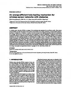
5.2. A Comparison Between EEDS, EAD, and LEACH Figure 9 shows a comparison between EEDS and EAD in terms of the number of live nodes vs time under different (1, 5, 10) data transmission periods. We observe that EEDS outperforms EAD. The time for the first node to die in EEDS is longer than in EAD. In EEDS, under one data transmission period, the time for the first node to die is about 87 seconds, while it is about 50 seconds when in EAD. An improvement of about 74% is achieved. On the other hand, increasing the number of data transmission period for a single tree and for the corresponding schedule will increase the time for the first node to die. This is very intuitive since building the tree and building the schedule consume energy. Using the same tree for the multiple data transmission period will save energy. When applying 10 data transmission periods, the time for the first node to die in EEDS is about 278 seconds, while it is about 60 seconds in the EAD protocol. The question that may arise here is: why don’t we use the same tree for the whole

October 2010


163


simulation time? In fact, we have examined the network under this assumption and we found that network life time has shrunk to 170 sec compared with our approach. It is very important to note that these network lifetime figures are functions of the data-sensing period that is considered very small in our simulation experiments. For example, considering the 10-data transmission periods example, the data-sensing period is 32.80 msec. In EAD protocol, since the gateways wait until they receive all the data packets from all their children, they will transmit their data packets to the sink at the end of the data transmission period. Therefore, their radios have to be ON for the whole data transmission period. This will consume a lot of energy; and they will die very early. On the other hand, since the application considered is periodic, the other nodes will be ON until they transmit their data packet. Then they will go to sleep until the time for the successive event. The gateway nodes will die earlier than other nodes. On the other hand, in EEDS, the gateways will sleep most of the time except during their scheduled time to receive and transmit. Therefore, their energy consumption will be smaller than gateways in EAD protocol. Therefore, gateways in EEDS stay alive for a longer time than gateways in EAD. In both protocols, when the gateways die, the remaining nodes will be isolated because they will not be able to communicate with the sink. The nodes that act as gateways in both protocols are limited to the closest existing nodes to the sink. These nodes act as gateways for the whole network lifetime and they die approximately at the same time. Therefore, in both protocols, the number of live nodes is stable around 100, then goes down very fast. Table 4. A Comparison Between EEDS and EAD in Terms of Throughput Data Transmission Period 1 5 10

EEDS 4569 18180 28350

EAD 4561 8085 8810

Improvement 0.17% 124.9% 221.8%

The improvement in the network lifetime in EEDS contributes to the increase in the number of data packets delivered to the sink (throughput). Table 4 shows a comparison between EEDS and EAD in terms of throughput. Since the network lifetime in EEDS is longer than in EAD, the sink will be able to receive more data packets from gateways for a longer time. Therefore, the aggregated throughput in EEDS is higher than the aggregated throughput in EAD. For example, with five data transmission periods, the aggregated throughput in EEDS is improved by about 124.9%.

Figure 10: Total consumed energy vs time (N=100)

Since the individual nodes in EEDS are scheduled to transmit and receive at specific time slots, they will be ON for these time slots, and they will be OFF for the remaining data transmission period. On the other hand, the nodes in EAD will be ON for the whole transmission period. The nodes in EEDS consume less energy than the nodes in EAD. Therefore, the total consumed energy in EEDS is smaller. As shown in Figure 10. It is clear that the total consumed energy in EEDS is much less than the energy consumed in EAD. For example, at t=50 seconds, and under one data transmission period, the total consumed energy in EEDS is about 100.4 J while it is about 154.5 in EAD. The energy consumption is reduced by 34.3%. Under five and ten data transmission periods, the energy consumption is reduced by 65.6% and 74.5%, respectively. Since gateways in EEDS take a longer time to die, the remaining 164


October 2010


nodes will be utilized for a longer time, which will extend the overall network lifetime and throughput. This interesting result argues for the effectiveness of the proposed algorithm EEDS. EEDS differs from LEACH in that a tree is connecting between nodes and the sink rather than sets of clusters connected to the sink via clusters’ heads. In addition, the data transmission between gateways and sink is performed using TDMA schedule rather than CSMA mechanism. To compare EEDS and LEACH protocols, we use the optimal number of clusters in LEACH as per [2] . For our network configuration, the optimal number of clusters is 4. Figure 11 shows a comparison between EEDS and LEACH in terms of the number of live nodes vs time. We observe that EEDS outperforms the LEACH under all data transmission periods. For example, under 10 data transmission periods, the network lifetime in EEDS is 330.7 seconds while it is about 246.7 seconds in LEACH. An improvement by 34.0% is achieved in EEDS. The improvement in the network lifetime is due to the savings in energy consumption in each node in EEDS.

Figure 11: Number of live nodes vs time

To compare the energy consumed by a node in LEACH and a node in EEDS, we note that in each protocol there are two types of nodes: head and non-head nodes in LEACH, leaf and non-leaf nodes in EEDS. In EEDS, the parent of a leaf node is always one of the nearest neighbors of the node. On the other hand, the parent of a non-head node in LEACH can be any head in the network because it is assumed that all nodes can hear each other. Although the parent of a node is the closest head, it may not be one of the nearest neighbors. It may be far away from the non-head node. Therefore, the transmission distance for a node in EEDS is less than in LEACH and the energy consumed due to transmission by a leaf node in EEDS is less. On the other hand, the head node in the LEACH protocol will consume more transmission energy than the nonleaf node in EEDS because the head node uses CSMA while the non-leaf node in EEDS is scheduled to transmit at a particular time slot. The head node in LEACH has to be ON and sense the channel for the whole data transmission period to get its turns for transmission, while the non-leaf node in EEDS will be ON only at its assigned time slot and will be OFF for the remaining data transmission period. In addition, the head node will transmit data packets directly to the sink, which may be far away from it, while the non-leaf node will transmit data packets to its parent that is very close to it. Regarding the energy consumed due to receiving data packets, the non-leaf node in EEDS consumes less energy than the head node in LEACH because the non-leaf node usually has a smaller number of children than the head node in LEACH. In LEACH, since it is assumed that any node can hear the transmission of all the nodes, and since there are few heads in the network, the number of children per head will be large. On the other hand, in EEDS, only the nearest nodes to the non-leaf node can join it. Therefore, the number of children per each non-leaf node will be small. Taking into account the consumed energy during transmission and reception, the total consumed energy in EEDS will be smaller than in LEACH. This is shown clearly in Figure 12. For example, with 10 data transmission periods, at t=50 seconds, the total consumed energy in LEACH protocol is about 47.6 J while it is about 26.12 J in EEDS (scheduled). The consumed energy is improved by about 45.1%. Furthermore, in EEDS, the

October 2010


165


overall consumed energy is less than 200 J, the initial energy in the network, while in the LEACH protocol it is 200 J for fewer throughputs.

Figure 12: Total consumed energy vs time

The improvement in the network lifetime improves the number of data packets delivered to the sink. Table 5 shows a comparison between EEDS and LEACH in terms of aggregated throughput over all the simulation times. For example, for the 5 data transmission period, the throughput in EEDS is improved by 29.4%. Table 5. The Aggregated Throughput in EEDS Compared With LEACH Protocol Data Transmission Period 1 5 10

Proposed Protocol (scheduled) 4569 18180 28350

LEACH

Improvement

2984 14045 25840

53.1% 29.4% 9.6%

Table 6 shows a summary of the improvement in EEDS compared with EAD and LEACH protocols for all metrics (network lifetime, throughput, energy consumed) under different data transmission periods. Table 6. A Summary of the Improvement in EEDS Compared With EAD and LEACH

Network Lifetime Energy Consumed (t=50 s) Throughput

One Data Transmission EAD LEACH 35.5% 61.9%

Five Data Transmission EAD LEACH 47.8% 251.4%

Ten Data Transmission EAD LEACH 36.0% 405.4%

39.1%

36.5%

65.6%

42.6%

74.5%

37.7%

0.17%

53.1%

124.9%

29.4%

221.8%

9.6%

6. CONCLUSION In this paper, we proposed an Energy Efficient Distributed Schedule-Based (EEDS) protocol for WSN. EEDS is intended for applications with periodic data traffic. In EEDS, the time frame is composed of rounds. Each round consists of three phases. In the first phase, an energy-aware tree is built, and then a TDMA schedule is constructed in a distributed manner in the second phase. Based on the built schedule, the node will transmit their data in the third phase. At the beginning of each round, the tree will be rebuilt and a new TDMA schedule will be constructed. The data transmission phase can be repeated several times in a single round. The main contributions of this work can be summarized as follows. Firstly, we modify the building tree protocol used in [29] such that a node will join the tree only if it has sufficient energy to enable it to work for the whole round. The energy is calculated assuming the worst case (i.e., the node will be a non-leaf node in the coming round and it will have eight children). Secondly, the node will transmit with the minimum energy such that its transmission will reach the closest neighbors only, which will reduce the consumed energy during transmission. Thirdly, a global TDMA schedule for data transmission is built in a distributed manner. Each non-leaf node in the tree, based on the information sent by its children, will build its own schedule for its surrounding children. Then it transmits its own

166


October 2010


information to its parent to help it in building its schedule and so on. Fourthly, the energy consumed by each node will be reduced since each node will be ON only for its transmission slot and for its receiving slot and will be OFF for the remaining slots. EEDS is examined under different network configurations and compared with EAD and LEACH protocols in terms of network lifetime, throughput and energy consumption. Compared with EAD protocol, the network lifetime in EEDS is improved by at least 67.3%. On the other hand, the energy consumption is also decreased by 34.4% to 74.5% and the aggregate throughput is significantly improved. On the other hand, compared with the LEACH protocol, the network lifetime in EEDS is improved by at least 33.3%., the energy consumption is also decreased by more than 33.3%, while the throughput is improved by 8.6 %–48.7%. We observed that the network lifetime is constrained by the gateway nodes (nodes connected directly to the sink). As a future work, we will modify EEDS to increase the number of candidate gateways and compare the modified protocol with other existing protocols. In addition, we need to study what is the optimal network size associated with each sink node. We observed also that increasing the number of data transmission phases in a single round would increase the network lifetime and throughput, and decrease energy consumption. We need to identify the optimal number of data transmission period in a single round for a specific network size. Finally, EEDS may suffer a longer delay in delivering data to the sink, which in turn may cause a packet drop especially if the delay caused by the EEDS overhead (i.e., building tree and schedule) is greater than the data period. ACKNOWLEDGMENT This work is supported by both KACST under project #117-28 and King Fahd University of Petroleum and Minerals, Dhahran, Saudi Arabia, under project IN-090022. REFERENCES [1] I. F. Akylidiz, W. Su, Y. Sankarasubramaniam, and E. Cayirci, “A Survey on Sensor Networks”, IEEE Personal Communications Magazine, August 2002, pp. 102–114. [2] W. R. Heinzelman, A. P. Chandrakasan, and H. Balakrishnan, “An Application-Specific Protocol Architecture for Wireless Microsensor Networks, IEEE On Wireless Communications Trans.”, 1(4)(2002), pp. 660–670. [3] J. Li and G. Lazarou, “A Bit-Map-Assisted Energy-Efficient MAC Scheme for Wireless Sensor Networks”, IPSN'04, April 2004, pp. 55–60. [4] S. Biaz and Y. D. Barowski, “GANGS: An Energy Efficient MAC Protocol for Sensor Networks”, ACMSE'04, April 2–3, 2004, pp. 82–87. [5] S. Mishar and A. Nasipuri, “An Adaptive Low Power Reservation Based MAC Protocol for Wireless Sensor Networks”, in IEEE International Conference on Performance, Computing, and Communications, 2004, pp. 731– 736, [6] S. Chung, S. Lee, and H. Yoon, “An Efficient TDMA Scheduling Scheme for Wireless Sensor and Actor Networks”, IEICE Trans. Commun., E91–B(6)(2008), pp.1886–1895. [7] M. D. Jovanovic and G. L. Djordjevic, “TFMAC: Multi-Channel MAC Protocol for Wireless Sensor Networks”, Telecommunications in Modern Satellite, Cable and Broadcasting Services, 2007. TELSIKS 2007. 8th International Conference on , Sept. 26–28, 2007, pp. 23–26. [8] L. Gong, “A Two Level TDMA Scheduling Protocol With Intra-Cluster Coverage for Large Scale Wireless Sensor Network”, IJCSNS International Journal of Computer Science and Network Security, 6(2B)(2007), pp.77–84. [9] G. Haigang, L. Ming, W. Xiaomin, C. Lijun, and X. Li, “An Interference Free Cluster-Based TDMA Protocol for Wireless Sensor Networks”, in Wireless Algorithms, Systems, and application , ISBN: 978-3-540-37189-2, 2006 , pp. 217–227 [10] S. Kumar, V. S. Raghavan, and J. Deng, “Medium Access Control Protocols for Ad Hoc Wireless Networks: A Survey”, Ad Hoc Networks, 4(2006), pp. 326–358. [11] M. Younis and S. Bushra, “Efficient Distributed Medium Access Arbitration for Multi-Channel Wireless Sensor Networks”, in Proceedings of the 32nd IEEE International Conference on Communications (ICC 2007), Glasgow, Scotland, UK, June 22–28, 2007, pp. 3666–3671. [12] O. Younis and S. Fahmy, “HEED: A Hybrid, Energy-Efficient, Distributed Clustering Approach for Ad Hoc Sensor Networks”, in IEEE Trans. on Mobile Computing, 3(4)(2004), pp. 366–379. [13] K. Sohrabi and G. J. Pottie, “Performance of a Novel Self-Organization Protocol for Wireless Ad Hoc Sensor Networks”, in Proceeding IEEE 50th Vehicular Technology Conf., 2, Sept. 19–22, 1999, pp. 1222–1226. [14] W. Ye, J. Heidemann, and D. Estrin, “Medium Access Control With Coordinated Adaptive Sleeping for Wireless Sensor Networks”, IEEE/ACM Transactions on Networking, 12 (3)(2004), pp. 493–506.

October 2010


167


[15] M. Stemm and R. H. Katz, “Measuring and Reducing Energy Consumption of Network Interfaces in Hand-Held Devices”, IEICE Transactions on Communications, E80-B(8)(1997), pp. 1125–1131. [16] K. Akkaya and M. Younis, “A Survey of Routing Protocols in Wireless Sensor Networks”, Elsevier Ad Hoc Network Journal, 3/3(2005), pp. 325–349. [17] P. Lin, C. Qiao, and X. Wang “Medium Access Control With a Dynamic Duty Cycle for Sensor Networks,” WCNC, Mar. 2004, pp. 1534–1539. [18] T. V. Dam and K. Langendoen, “An Adaptive Energy-Efficient MAC Protocol for Wireless Sensor Networks”, ACM Sensys’03, Nov. 2003, pp. 171–180. [19] C. Intanagonwiwat, R. Govindan, and D. Estrin, “Directed Diffusion: A Scalable and Robust Communication Paradigm for Sensor Networks”, in Proceedings of the 6th Annual ACM/IEEE International Conference on Mobile Computing and Networking (MobiCom'00), Boston, MA, August 2000, pp. 56–67. [20] C. Schurgers and M. B. Srivastava, “Energy Efficient Routing in Wireless Sensor Networks”, in The MILCOM Proceedings on Communications for Network-Centric Operations: Creating the Information Force, McLean, VA, 1, Oct. 28–31, 2001, pp. 357–361. [21] D. Braginsky and D. Estrin, “Rumor Routing Algorithm for Sensor Networks”, in Proceedings of the First Workshop on Sensor Networks and Applications (WSNA), Atlanta, GA, October 2002, pp. 22–31. [22] R. Shah and J. Rabaey, “Energy Aware Routing for Low Energy Ad Hoc Sensor Networks”, in Proceedings of the IEEE Wireless Communications and Networking Conference (WCNC), Orlando, FL, 1, March 17–21, 2002, pp. 350– 355. [23] W. Heinzelman, J. Kulik, and H. Balakrishnan, “Adaptive Protocols for Information Dissemination in Wireless Sensor Networks”, in Proceedings of the 5th Annual ACM/IEEE International Conference on Mobile Computing and Networking (MobiCom’99), Seattle, WA, August 1999, pp. 174–185. [24] S. Lindsey and C. S. Raghavendra, “PEGASIS: Power Efficient GAthering in Sensor Information Systems”, in Proceedings of the IEEE Aerospace Conference, Big Sky, Montana, 3, March 2002, pp. 1125–1130. [25] S. Lindsey, C. S. Raghavendra , and K. Sivalingam, “Data Gathering in Sensor Networks Using the Energy*Delay Metric”, in Proceedings of the IPDPS Workshop on Issues in Wireless Networks and Mobile Computing, San Francisco, CA, April 2001, pp. 2001–2008. [26] A. Manjeshwar and D. P. Agrawal, “PTEEN: A Hybrid Protocol for Efficient Routing and Comprehensive Information Retrieval in Wireless Sensor Networks”, in Proceedings of the 2nd International Workshop on Parallel and Distributed Computing Issues in Wireless Networks and Mobile Computing, Ft. Lauderdale, FL, April 2002, pp. 195–202. [27] V. Rodoplu and T.H. Ming, “Minimum Energy Mobile Wireless Networks”, IEEE Journal of Selected Areas in Communications, 17(8)(1999), pp. 1333–1344. [28] Y. Yu, D. Estrin, and R. Govindan, “Geographical and Energy-Aware Routing: A Recursive Data Dissemination Protocol for Wireless Sensor Networks”, UCLA Computer Science Department Technical Report, UCLA-CSD TR01-0023, May 2001. [29] A. Boukerche, X. Cheng, and J. Linus, “A Performance Evaluation of a Novel Energy-Aware Data-Centric Routing Algorithm in Wireless Sensor Networks”, Wireless Networks, 11(2005), pp.619–635, [30] S. R. Madden, M. J. Franklin, J. M. Hellerstein, and Wei Hong, “TinyDB: An Acquisitional Query Processing System for Sensor Networks”, ACM Transaction on Database Systems, 30(1)(2005), pp. 122–173. [31] Sensor Modules, http://www.xbow.com, accessed , October 2008.

168


October 2010