An Energy Efficient Protocol for Wireless Sensor Networks Andrea Depedri, Alberto Zanella and Roberto Verdone IEIIT-BO/CNR, DEIS-University of Bologna, Italy Email:
[email protected] 100 90 80 70 60 SENSORS
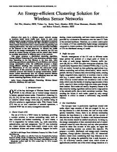
50
Meters [m]
Abstract— Networking together hundreds or thousands of cheap microsensor nodes allows users to accurately monitor a remote environment by intelligently combining the data from the individual nodes. These wireless networks require robust routing protocols that are energy efficient and provide low latency. Starting from the basic idea of classical LEACH (Low Energy Adaptive Clustering Hierarchy), in this paper we introduce some innovations in the algorithm giving origin to LEACH-B. LEACHB presents a new strategy of cluster heads election and cluster formation. Our results show that LEACH-B optimizes system lifetime in a large range of situations and applications.
40 30 20
Keywords: Sensor networks, wireless networks, routing algorithms, energy saving strategies. I. I NTRODUCTION In ad hoc networks, devices are required to self-organize themselves into a network without previously established infrastructure. Advances in sensor technology, low-power electronics, and low-power radio frequency (RF) design have enabled the development of small, relatively inexpensive and low-power sensors, called microsensors, that can be connected via a wireless network. These wireless microsensor networks, which constitute a subclass of ad hoc networks, represent a new paradigm for extracting data from the environment and enable the reliable monitoring of a variety of environments for applications that include surveillance, machine failure diagnosis, and chemical/biological detection. An important challenge in the design of these networks is that two key resources, communication bandwidth and energy, are significantly more limited than in a tethered network environment. These constraints require innovative design techniques to use the available bandwidth and energy efficiently [1], [2]. A recent protocol architecture that optimizes the energy efficiency in microsensor networks is Low Energy Adaptive Clustering Hierarchy (LEACH) [3], [4]. LEACH considers communications between sensor nodes randomly distributed in a fixed square area, and an external receiver. It includes distributed cluster formation technique, that enables self-organization of large numbers of nodes, algorithms for adapting clusters and rotating cluster head positions to evenly distribute the energy load among all nodes. In this paper, starting from the basic idea of LEACH [3], [4], we propose a new routing strategy, denoted as LEACH-B; the main characteristics of our performance analysis are: 1) We characterize in a better way the transceiver than how it was done in [3], [4] with data taken from [5].
10 0 −50 0
−40
−30
−20
−10
0
10
20
30
40
50
FINAL RECEIVER
−20 −40 −50
−40
−30
−20
−10
0
10
20
30
40
50
Meters [m]
Fig. 1.
Reference scenario
2) We consider a decentralized algorithm of cluster formation, in which sensor nodes only know their own position and the position of the final receiver, and not the position of all sensors. 3) With our model, the optimal number of cluster heads depends also on the energy dissipated for broadcast packets. 4) We propose a new adaptive strategy to choose the cluster head election’s frequency. 5) We propose a new idea for cluster formation, which considers the total path energy dissipation and not only the energy dissipated in the path between the node and his cluster head. 6) We provide first results also considering a fading channel. Our work has been inspired by a specific application: the monitoring of a big car-park in which sensors, distributed in the area, interact to communicate to an external receiver (mounted over a car) the better way to reach the closest free place. We assume that sensors are equipped with a limited energy battery. Abstracting from this application we consider a less specific one with NT OT = 100 sensors randomly distributed in a square area (side M = 100m) and an external receiver far away from the sensors’ area. This scenario has been used as reference and is shown in figure 1.
l-bit packet
S
APPT
E
AE
APPR
Fig. 2.
Gt
PE =
d
l-bit packet
U
where PAP PT includes the power dissipated in the oscillator, frequency synthesizer, mixers, filters, baseband processing,. . . etc. PE is the power needed by the transmitter for providing an acceptable signal to noise ratio, Eb /N0 , at the receiver. PE can be computed as
R
AR
PRX AE A0 AR Gt ηamp Gr
(5)
where PRX is the receiver sensitivity, ηAmp is the transmitter amplifier efficiency. The receiver sensitivity can be further written as
Gr
PRX = ρm FRX kT0 Beq
Transmission system block diagram.
II. P HYSICAL A SPECTS In this section we describe the radio propagation channel and the energy dissipation in the transmitter and in the receiver. In figure 2 we can see the scheme of the transceiver, composed of a transmitting and a receiving part. The block AP PT is composed by a coder, a modulator and an upconverter; consequently the block AP PR is composed by a down-converter, a demodulator and a decoder. S and U are respectively the source of bits and the final user. E and R represent the emitter and receiver, respectively. The blocks AE , AR represent the attenuations due to the connections of transmitting and receiving antennas, respectively. Finally Gt and Gr denote the antennas’ gains and d denotes the distance between transmitter and receiver. A. Characterization of Radio Channel: free space loss We consider a propagation channel model in which pathloss attenuation A0 is described as follows: µ ¶ µ ¶α 1 d A0 = (1) L0 d0 where 1/L0 is the Path-loss attenuation at d0 meters, d0 being a refernce distance, α is the path-loss exponent. By setting µ ¶ µ ¶2 µ ¶2 1 4π (4π)ft = = , (2) L0 λ c where λ [m] is the Wavelength of the transmitted signal, ft [Hz] is the frequency of transmission, and c [m/s] is the speed of light, we can consequently rewrite (1) as: µ ¶2 µ ¶α (4π)ft d A0 = . (3) c d0 B. Energy Characterization for the Transmitting part
(6)
where ρm is the real minimum required signal to noise ratio at the receiver for an acceptable Eb /N0 , FRX is the receiver noise figure (numeric), k is the Boltzman constant, T0 is the floor thermal noise temperature and Beq is the receiver equivalent noise bandwidth. By setting Gt Gr GAnt = , (7) AE AR expression (5) can be written as follows: µ ¶2 ³ ´ α (4π)ft d ρm FRX kT0 Beq c d0 PE = (GAnt ) (ηAmp )
(8)
Now, if we approximate the minimum amount of energy per bit required at the transmitter by ET X =
PT X PAP PT PE = + Br Br Br
(9)
where Br is the raw bit rate in bits per second, we can easily write the expression of the energy dissipated by the transmitter to send a packet of l bits as µ ¶ PAP PT PE ETl = lET X = l + = l (EAP PT + β(d)) , Br Br (10) where β(d) = PE /Br is a function of d through PE . C. Energy Characterization for the Receiving part The power dissipated in the electronics of the receiver is represented as PR + PAP PR , where PR and PAP PR represent the power dissipated in the receiver front-end and at AP PR , respectively. To receive a message, the energy per bit dissipated in the receiver is:
We start our analysis with the assumption that all sensors in the network are simple and inexpensive but have a power control mechanism to vary the amount of transmit power. For every transmission the minimum power required by the transmitter can be written as (all powers in Watts):
Consequently to receive a l bit packet the energy dissipation is:
PT X = PAP PT + PE
ERl = lERX .
(4)
ERX =
PR + PAP PR . Br
(11)
(12)
III. R EFERENCE A LGORITHMS Many algorithms have been proposed for ad hoc sensor networks. As reference we consider three of these algorithms: Multi-Hop (MH), Direct, and Classical LEACH or LEACHA [3], [4], [5]. These algorithms are briefly described in this section. First of all we have to explain how the time axis is considered in our analysis. We divide the time axis in rounds. Each round starts with the request of the final receiver to know the actual situation of the monitored environment. Upon reception of this request, all sensors in the network reveal the observed phenomenon and send their information packet at the external receiver. When all sensors have sent their message the round is closed. A. Multi-Hop In MH the observed area is divided into a fixed number of zones, as shown in figure 3 (four zones). For each round, the sensors of zone number 4, send their packet to a node in zone number 3, and so on until they reach a sensor in zone number 1. The sensors in zone 1, at last, send all packets received and their own packet to the final receiver. It is quite clear that these last sensors are very penalized, energetically speaking, because they have to transmit a large number of packets. Consequently in MH the first nodes to finish their energy are the closest ones to the final receiver. 120
100
ZONE 4
80
Meters [m]
ZONE 3
ZONE 2
20
ZONE 1 0 0 −20 −40 −50
−40
−30
−20
−10
0
10
20
30
40
50
Meters [m]
Fig. 3.
IV. LEACH-B: T HE P ROPOSED A LGORITHM The new algorithm we propose in this section, named LEACH-B, differs for some aspects and assumptions from LEACH-A [3], [4]. First of all we consider a decentralized algorithm of cluster formation, in which sensor nodes only know their own position and the position of the final receiver, and not the position of all sensors. Moreover we do not consider the aggregation process of data at cluster head because it is not useful for many applications (e.g. car-park). In this section we reanalyze the different phases of LEACH-A giving more emphasis to the innovations and advantages introduced by LEACH-B. A. Optimum Number of Clusters
60
40
cluster head. All non-cluster head nodes transmit their data to the cluster head, while the cluster head node receives data from all the cluster members, performs multiplexing functions on the data (e.g., data aggregation), and transmits data to the remote receiver. Therefore, being a cluster head node is much more energy intensive than being a non-cluster head node. If the cluster heads were chosen a priori and fixed throughout the system lifetime, these nodes would quickly use up their limited energy. Once the cluster head runs out of energy, it is no longer operational, and all the nodes that belong to the cluster lose communication ability. Thus, LEACH incorporates randomized rotation of the high-energy cluster head position among the sensors to avoid draining the battery of any one sensor in the network. In this way, the energy load of being a cluster head is evenly distributed among the nodes. The operation of LEACH is divided into rounds. Each round begins with a set-up phase when the clusters are organized, followed by a steady-state phase when data are transferred from the nodes to the cluster head and on to the final receiver.
Multi-Hop Model
B. Direct This model is very easy. For each round all sensors send their information packet directly to the final receiver. It is clear that in this case the farthest nodes have a larger energy dissipation because of their distance from the receiver. With Direct then the farthest nodes have the lowest battery duration. C. LEACH-A: Classical LEACH As described in [3], [4], with LEACH the nodes organize themselves into local clusters, with one node acting as the
ˆ is chosen As in [3], [4], the optimum number of clusters N in order to minimize the total transmission energy; however, in this paper for each cluster head we consider also the energy dissipated to send the broadcast packet for giving notice to other nodes of its position and role. Furthermore, as we said before, all cluster heads have to retransmit towards the final receiver all packets they receive from the members of their cluster. We assumed that there are NT OT nodes distributed ˆ clusters, there uniformly in a M × M region. If there are N ˆ nodes per cluster (one cluster head are on average NT OT /N ˆ ) − 1 non-cluster head nodes). Each cluster and (NT OT /N head dissipates energy retransmitting packets of the other sensors to the final receiver, transmitting their own packet and transmitting the broadcast packet. Consequently, the energy dissipated by the cluster head at round ti is ¶ µ NT OT − 1 (EAP PT + β(dCH−F R )α ) ECH (ti ) = l ˆ N | {z } Retransmitted
packets
+ l(EAP PT + β(dCH−F R )α ) | {z } Own
packet
(13)
+ l(EAP PT + β(dbroadcast )α ) | {z } Broadcast
packet
where dCH−F R is the distance between the cluster head and the external receiver and dbroadcast is the distance between the cluster head and the farthest point of the observed area. Each non-cluster head node only has to transmit its packet to the cluster head and so the energy dissipated for each round values EN CH (ti ) = lEAP PT + lβ(dp−CH )α
(14)
where dp−CH is the distance between the p-th node and the cluster head. As developed in [3] the expected squared distance from the a general node p to the cluster head is given on average by E[d2p−CH ] =
M2 , ˆ 2π N
so that (14) can be approximated by
Ã
EN CH (ti ) ' lEAP PT + lβ
M p ˆ 2π N
(15) !α .
(16)
For each round, the total transmission energy dissipated in a cluster is on average: µ ¶ NT OT Ecluster−T X (ti ) = ECH (ti ) + − 1 EN CH (ti ). ˆ N (17) Setting the approximation µ ¶ NT OT NT OT −1 ' , (18) ˆ ˆ N N expression (17) becomes µ ¶ NT OT Ecluster−T X (ti ) ' ECH (ti ) + EN CH (ti ). (19) ˆ N Finally the total energy dissipated for each round in the network has the following expression ˆ Ecluster−T X (ti ); ET OT −T X (ti ) = N
(20)
using the previous expressions, we get ˆ l(EAP P + β(dbroadcast )α ) N T µ 2 ¶α 2 M ˆ + lNT OT β + K, (21) ˆ 2π N ˆ is a term that does not depend on N ˆ . Considering that where K EAP PT ¿ β(dbroadcast )α , we can find the optimum number of clusters by setting the derivative of ET OT −T X performed ˆ , to zero. In this case we obtain: with respect to N s µ ¶α α +1 1 NT OT α M 2 2 ) ( 2 ˆ . (22) N= 2 2π (dbroadcast )α ET OT −T X (ti ) '
We can notice that each sensor can determine its own optimum number of clusters. This value depends on the total number of sensors in the network, on the exponent of path-loss, on the
dimension of the network and on the distance of broadcast packet. It no longer depends on the distance between the cluster head and the final receiver like instead was in LEACHA. B. Cluster Head Selection Algorithm LEACH (A or B) forms clusters by using a distributed algorithm, where nodes make autonomous decisions without any centralized control. Our goal is to design a cluster formation algorithm such that there are, on average, a certain number ˆ , during each round. In addition, if nodes begin of clusters, N with equal energy, our goal is to try to evenly distribute the energy load among all the nodes in the network so that there are no overly-utilized nodes that will run out of energy before the others. As being a cluster head node is much more energy intensive than being a non-cluster head node, this requires that each node takes its turn as cluster head. As explained in [3], [4], initially, when clusters are being created, each node decides whether or not to become a cluster-head for the current round. Ensuring that all nodes are cluster heads the same number of times requires each node to be a cluster head ˆ rounds on average. We consider Cp (ti ) the once in NT OT /N indicator function determining whether or not node p has been ˆ c ) rounds a cluster head in the most recent (r mod bNT OT /N (i.e. Cp (ti ) = 0, if node p has been a cluster head and one otherwise). r is a counter incremented at each round, when r ˆ c−1 is set to zero. The decision to become reaches bNT OT /N or not a cluster head is made by node p choosing a random number between 0 and 1. If the number is less than a threshold Tp (ti ), the node becomes a cluster head for the current round. The threshold is set as: ( ¦¢ : Cp (ti ) = 1; ¡ Nˆ ¥ N T OT ˆ N − N r mod T OT ˆ Tp (ti ) = (23) N 0 : Cp (ti ) = 0. ˆ is a fixed value and it In conventional LEACH (LEACH-A) N is determined a priori. In LEACH-B we introduce an adaptive ˆ that considers the real energy dissipation of variation of N each sensor the last time it has assumed the role of cluster head. If we consider an average situation, each cluster head has to ˆ packets to the final receiver. We set: send NT OT /N µ ¶ µ ¶ NT OT NT OT ECH−f ar = − 1 (lER ) + (lEAP PT ) ˆ ˆ N N µ ¶ NT OT + (lβ(df ar )α ) , (24) ˆ N ¶ µ ¶ NT OT NT OT − 1 (lER ) + (lEAP PT ) ˆ ˆ N N µ ¶ NT OT + (lβ(dclose )α ) . (25) ˆ N µ
ECH−close
=
where df ar and dclose are the distances between final receiver and the farthest point of the network and the closest one.
TABLE I Parameters of reference scenario
Starting from the average of these energies ECH−f ar + ECH−close , (26) 2 we fix two different thresholds (ECH−limSU P ) and (ECH−limIN F ) as follows: ECH−avg =
(27)
ECH−limIN F = ECH−avg − 0.6 × ECH−avg .
(28)
If the energy dissipated by the node p the last time it assumed the role of cluster head is larger than ECH−limSU P , the value ˆ used by node p, Nˆp , is decreases by 1, so that this node of N will become less frequently cluster head in the next rounds. At the opposite, if this energy is smaller than ECH−limIN F Nˆp = Nˆp − 1 and this node will become more frequently cluster head in the next rounds. Finally if the energy dissipated is between the two thresholds the value of Nˆp does not change. In this way we obtain a better distribution of the energetic expensive role of cluster head among all nodes in the network. C. Cluster Formation Algorithm Each node that has elected itself cluster head for the current round, broadcasts a message of notification to the rest of the nodes. The non-cluster head nodes must keep their receivers on during this phase of set-up to hear the advertisements of all the cluster head nodes. After this phase is complete, each noncluster head node decides the cluster to which it will belong for this round. In LEACH-A the non-cluster head sensor elects its cluster head choosing the minimum energy path between the node and the different possible cluster heads. In LEACH-B we introduce a new strategy to form the cluster. Each node chooses its cluster head evaluating the energy dissipated in the complete path between itself and the final receiver, passing by the cluster head. This is possible because each node in the network knows its position and the position of the external receiver. D. Data transmission and Multiple Access As assumed in [3], for each round a TDMA scheme is created by cluster heads to receive and retransmit the packets to the final receiver. The Multiple Access aspects, though fundamental, are not considered in this paper. V. N UMERICAL R ESULTS In this section we show the numerical results obtained with our simulator (implemented in C++). We start from the analysis of a reference scenario and then illustrate the performance of LEACH-B when varying some parameters of the scenario. A. Reference Scenario In table I we illustrate the parameters that characterize our network in the reference case. We have evaluated the performance of the algorithms proposed in terms of system lifetime. The system lifetime is defined
Value 2.4 GHz 15 dB (31.623) 0.2 m −20 dB (0.01) 1.0 Mb/s 1.03E + 6 Hz 6 dB (3.981) 0.8 2.3 3.63E − 3 W 11.13E − 3 W 0m −50 m 100 m 100 5.0 J 50 bit 4
as the time in which the first sensor in the network uses up its energy. In figure 4 we show the performance of the four algorithms considered in this paper, evaluated with reference parameters. 105
100
95
Number of sensors still alive
ECH−limSU P = ECH−avg + 0.6 × ECH−avg ,
Parameter ft ρm d0 GAnt Br Beq FRX ηamp α PAP PT PAP PR + PR X-Final Receiver Y-Final Receiver Network Side Number of Sensors Battery Energy Bits per packet Number of zones (Only MH)
DIRECT
MH
90
LEACH−B
85
80
LEACH−A
75
70
65 0
10
20
30
40
50
60
70
80
90
Rounds (X1000)
Fig. 4.
Performance in the reference scenario
In this situation with the receiver 50m away from the network we can see that LEACH-A and LEACH-B show similar performance in terms of system lifetime but they largely outperform both Direct and MH. B. Sensitivity to parameters We have investigated LEACH-B performance with respect to LEACH-A by varying many parameters: the distance of the final receiver, the side of the network, the number of sensors, the path-loss exponent, the thresholds etc. In figure 5 we can see that LEACH-B outperforms LEACH-A when the distance of the final receiver is less than 50m and the advantages grow up when decreasing this distance. Figure 6 shows that performance of LEACH-B is better than
150
We have proposed a new idea for cluster’s formation, which considers the total path energy dissipation between the node and the final receiver. • We have also considered the energy dissipated by cluster heads to send their broadcast packets. Our simulations have shown that LEACH-B outperform LEACH-A in a large class of situations and applications and in particular when: • The final receiver is closer to the sensors. • The deterministic attenuation due to the path-loss has a value of α larger than 2.5.
Round in which first node dies (X1000)
•
DIRECT MH LEACH−B LEACH−A
100
50
0 −100
−90
−80
−70
−60
−50
−40
−30
−20
−10
0
ACKNOWLEDGEMENTS
Y−Final Receiver [m]
Fig. 5.
This work is carried out in the framework of the Project VICOM (Virtual Immersive Communications), funded by MIUR, Italy. The Authors would like to thank the local Project responsible, Prof. Oreste Andrisano, for the motivation given to the work.
Variation of final receiver distance
6
10
Round in which the first node dies [dB]
DIRECT MH LEACH−A LEACH−B
R EFERENCES
5
10
4
10
3
10
2
10
2
2.1
2.2
2.3
2.4
2.5
2.6
2.7
2.8
2.9
3
Path−loss Exponent [α]
Fig. 6.
Variation of path-loss exponent
LEACH-A when the path-loss exponent α is larger than 2.5. Moreover figure 6 shows an extremely linear development of all curves with respect to variation of α. Finally, we implemented a propagation channel where a lognormal random variable is associated to the loss of each packet transmission. For the sake of conciseness, we do not give details in this paper. However, it is worthwhile mentioning that the conclusions drawn by previuos analysis are still valid even though the absolute values of battery durations are in general shorter owing to the margins introduced in the link budgets, needed to counteract random fluctuations. VI. C ONCLUSIONS In this paper we have proposed a new algorithm for sensor networks that minimizes global energy usage by distributing the load to all the nodes at different points in time. Our algorithm is based on classical LEACH but propose many important innovations and improvements that can be briefly resumed as follows: • We have proposed a new adaptive strategy to choose cluster heads and to vary their election’s frequency considering the dissipated energy.
[1] Xiaoyan Hong, Kaixin Xu, and Mario Gerla, “Scalable Routing Protocols for Mobile Ad Hoc Networks”, IEEE Network July/August 2002. [2] Ian F. Akyildiz, Weilian Su, Yogesh Sankarasubramaniam, and Erdal Cayirci, “A Survey on Sensor Networks”, IEEE Communications Magazine August 2002. [3] Wendi B. Heinzelman, Anantha P. Chandrakasan, and Hari Balakrishnan, “An Application-Specific Protocol Architecture for Wireless Microsensor Networks”, IEEE Trans. on Wireless Comm., Vol. 1, No. 4, Oct. 2002. [4] W. Heinzelman, A. Chandrakasan, and H. Balakrishnan, “Energy-efficient routing protocols for wireless microsensor networks”, in Proc. 33rd Hawaii Int. Conf. System Sciences (HICSS), Maui, HI, Jan. 2000. [5] Priscilla Chen, Bob O’Dea, Ed Callaway Motorola Labs, “Energy Efficient System Design with Optimum Transmission Range for Wireless Ad Hoc Networks”, IEEE International Conference on Comm. (ICC 2002), Vol. 2, pp. 945-952, 28 April -2 May 2002. [6] C. -C. Chiang and M. Gerla, “Routing and Multicast in Multihop, Mobile Wireless Networks”, Proc. IEEE ICUPC 97, San Diego, CA, Oct. 1997. [7] M. Gerla, X. Hong, and G. Pei, “Landmark Routing for Large Ad Hoc Wireless Networks”, Proc. IEEE GLOBECOM 2000, San Francisco, CA, Nov. 2000. [8] Bulusu et al., “Scalable Coordination for Wireless Sensor Networks: SelfConfiguring Localization Systems”, ISCTA 2001, Ambleside, U.K., July 2001. [9] J. M. Rabaey et al., “PicoRadio Supports Ad Hoc Ultra-Low Power Wireless Networking”, IEEE Comp. Mag., 2000, pp. 4248. [10] S. Corson and J. Macker, “Mobile Ad hoc Networking (MANET): Routing Protocol Performance Issues and Evaluation Considerations”, RFC 2501, Jan. 1999.