Aug 6, 1996 - of visualization methods, such as graphs, text, graphics objects, etc. .... variables into the Explorer data types cxParameter or cxLattice and back. ... Therefore, on top of this API a Data I/O library was defined, which is tuned to ...
An Environment for Computational Steering Jarke J. van Wijk 1 2 Robert van Liere 2 August 6, 1996
Abstract Computational Steering is the ultimate goal of interactive simulation: researchers change parameters of their simulation and immediately receive feedback on the effect. We present a general and flexible environment for computational steering. Within this environment a researcher can easily develop user interfaces and 2-D visualizations of his simulation. Direct manipulation is supported, and the required changes of the simulation are minimal. The architecture of the environment is based on a Data Manager that takes care of centralized data storage and event notification, and satellites that produce and visualize data. One of these satellites is a graphics tool to define a user interface interactively and to visualize the data. The central concept here is the Parametrized Graphics Object: an interface is built up from graphics objects whose properties are functions of data in the Data Manager. The scope of these tools is not limited to computational steering, but extends to many other application domains. Keywords: Visualization, computational steering, interaction, direct manipulation.
1
Introduction
1.1 Computational Steering Scientific Visualization has become a major research area since 1987, when the influential report of the NSF [1] was published. In recent years many new methods, techniques, and packages have been developed. Most of these developments are limited to post-processing of data-sets. Usually the assumption is made that all data is generated first and that next the researcher iterates through the remaining steps of the visualization pipeline (selection, filtering, mapping, and rendering) to achieve insight in the generated data. Hence, the interaction with the simulation is limited. Marshall et al. [2] distinguish two alternatives to this post-processing approach to visualization. The first step to more interaction with the simulation is with tracking. After each time-step of the simulation the resulting data for that time-step is sent into the visualization pipeline and can be inspected. If the researcher considers the results invalid, then the simulation can be stopped at an early stage, and restarted with a different set of input parameters. The next step, Computational 1 2
Netherlands Energy Research Foundation ECN, P.O. Box 1, 1755 ZG Petten, The Netherlands. Centrum voor Wiskunde en Informatica, P.O. Box 4097, 1009 AB Amsterdam, The Netherlands.
1
Steering goes a lot further, and can be considered as the ultimate goal of interactive computing. Computational steering enables the researcher to change parameters of the simulation while the simulation is progressing. According to Marshall et al. [2] : "Interaction with the computational model and the resulting graphics display is fundamental in scientific visualization. Steering enhances productivity by greatly reducing the time between changes to model parameters and the viewing of the results." Our aim is to provide researchers with a Computational Steering Environment (CSE ) that encourages exploratory investigation by the researcher of his simulation. In the following subsections we sum up the requirements, we discuss existing solutions, and give an overview of the remainder of this paper, in which we present our solution.
1.2 Requirements The data-flow between the researcher and his simulation via a CSE is shown in figure 1. The researcher can enter new values for parameters, and views visualizations of the resulting data. Hence, input widgets such as text-fields, sliders, and buttons must be provided, as well as a variety of visualization methods, such as graphs, text, graphics objects, etc. With such objects input and output are separated. For more direct control, objects must be provided that allow for two-way communication: both input and output. It must be possible to select and drag visualization objects, thereby directly controlling parameters of the simulation. In other words, direct manipulation must be provided. The simulation receives from the CSE new parameter values, and sends newly calculated results to the CSE . We assume that the simulation can handle changes of parameters on the fly, and that it can provide meaningful intermediate results within a time-interval that is acceptable to the researcher. The concept of direct manipulation has a counterpart in the interface between CSE and simulation. Some variables, typically state-variables, are continuously updated by the simulation, but can also be changed from outside of the simulation.
Researcher graphical input
direct manipulation
animation
Computational Steering Environment
parameters
state variables
results
Simulation
Figure 1: Data flow between researcher, CSE , and simulation
As an example of an interface with a high degree of interaction, consider figure 2. This shows an interactive graphics interface to a simulation of a set of bouncing balls in two dimensions. The balls are depicted as circles, each with a small red line that indicates the direction and magnitude 2
of its velocity. For every time step the simulation calculates the position and velocity of all balls. Various control-parameters such as the size of the balls, damping, attraction, a constant field-force, can be set. This can be done via sliders, by typing, or by dragging the arrows. The positions of the balls (state-variables) are continuously updated by the simulation, but can also be changed by the researcher by dragging their graphical representations to other positions. This figure is a screen-dump of a result of the CSE presented in this paper. In section 4.1 we come back to this example and show how it was defined.
Radius r
0.125
Contact force Fc d 2500
Contact damping Fcd velocity
0.000
Damping
velocity Fd
Time
Field force
0.125
Synchronous t = 47.882 dt = 0.005
Asynchronous
Attraction -0.20
Fa
Ekin = 0.06340
0.005
0.00
Figure 2: Simulation of bouncing balls
The researcher must be enabled to create and to refine the interface to the simulation easily and incrementally. The process of achieving insight via simulation is an incremental process. For all stages of the visualization pipeline (from simulation to rendering) the cycle specification, implementation, application is continuously reiterated. In the process of gaining insight via computational steering, a researcher typically wants to look at and to control other, possibly new variables, and to visualize them in different ways. The CSE must be able to deal with multiple processes simultaneously. There are three reasons for this: First, it must be possible to integrate existing tools, such as special purpose packages for grid-editing or visualization, into the CSE . Second, a simulation is often built up of several processes running on distant compute servers. Third, it would be convenient if several researchers could view and control the data simultaneously. The final requirement concerns the underlying data model and the amount of data within the CSE . The type of data to be handled depends very much on the type of simulation, and therefore can vary from simple scalar data to large, three-dimensional, time-dependent vector and tensor field data-sets. The underlying data model must be flexible enough to support a wide range of data types and data quantities. 3
1.3 Related work An optimal result for the researcher can be achieved if we build a complete system, incorporating handling of input, output, as well as the simulation, using basic graphics libraries, such as for instance IRIS GL, or PHIGS. Typical examples are flight-simulators and packages for mechanical engineering. This approach requires a large effort and considerable experience, and often leads to an inflexible system with fixed functionality. Thus, the requirement for easy modification by the researcher is violated. However, if the application is time-critical and has wide-spread use, the gain can be worth the cost. Given the set of requirements, how can we realize a more general solution, i.e. an environment rather than a turn-key system ? Basically, three approaches can be taken: consider the design and implementation of a CSE as a graphics problem, and extend a basic graphics library; consider it as a user interface problem and extend the functionality of a User Interface Management System (UIMS); consider it primarily as a visualization problem, and extend an application builder. All these approaches have been pursued. An exhaustive treatment would require far more space then is available here, because very many related approaches, techniques and concepts exist. We limit ourselves therefore to some relevant examples. Graphics libraries typically offer only low level functionality. To simplify the definition of interactive applications with direct manipulation, graphics libraries can be enhanced with higher level interactive objects. With this approach a tight coupling of application objects and interaction objects can be ensured. For example, the Inventor toolkit [3] provides an object-oriented library which simplifies the development of interactive graphics applications. Van Dam et al. [4] take this a step further. They describe an extensible system that primarily aims at the integration of a variety of simulation and animation concepts in the graphics toolkit. Objects may have geometric, algorithmic, or interactive properties. Objects may send messages to each other which, after being stored in the object, can be edited. The authors show how collision detection [5], constraints and deformation [6] are handled within this framework. Various UIMS’s have been described that provide support for coupling the application (represented by a set of application objects) and the user interface [7, 8, 9]. User interface and application designers can develop their parts independently and have the UIMS manage the dialogue layer to integrate the two parts. Some UIMS’s allow users to specify direct manipulation interfaces through WYSIWYG editors. An example is the Peridot system [10], which allows non-programmers to create sophisticated interaction techniques. With the help of graphical constraints, Peridot allows a user to draw graphical objects of the user interface. The user provides the behavior of these graphical objects with a technique called programming by example. This results in Peridot generating parameterized procedures which can, in turn, be linked in or interpreted by the application program. Application builders have emerged as a flexible solution for scientific visualization. The users are provided with a set of modules, which can be connected and extended to rapidly prototype applications and reconfigure existing ones. Some researchers have discussed the use of computational steering [11, 12, 2] in this context. With the current generations of such systems the user can define user interface panels. The simulation has to be included as a module. The 4
extension of such systems with direct manipulation has been discussed in [13]. In general, the implementation of direct manipulation is cumbersome, because in data flow environments the relation between the original data and the geometric objects in the visualization is not known. Finally, a novel approach to exploratory visualization has been taken in VIEW [14]. The key idea of VIEW is a very tight coupling of geometry with an underlying database. The VIEW system allows researchers to interact directly with the visualization. Researchers can select tools for the visualization of their data. This allows and encourages researchers to experiment and explore the underlying data spaces. Scripting languages are used for defining new tools. All approaches discussed have a value on their own right. However, we feel that none satisfies all CSE requirements simultaneously. The extensions discussed of basic graphics libraries are very convenient for graphics application programmers, but are not directly suitable for use by researchers. The visualization of data is outside the scope of current UIMSs. Application building environments do not provide direct manipulation, which we consider as an important issue for computational steering. In the VIEW system new visualization tools must be specified via a specialized scripting language. Here the graphics objects, and the relations between graphics objects, data, and user actions are specified.
1.4 Overview In the following sections we present an environment for Computational Steering that does satisfy our requirements. The space available here does not allow for a detailed treatment, a more extensive description can be found in [15]. In section 2 we give an overview of the architecture. The central component is a Data Manager, which is responsible for managing data storage and process communication. In section 3 a general tool for graphical input and output is described. We have taken the approach of extending low level graphics. We use the notion of a Parametrized Graphics Object (PGO ) as the main concept, and a graphics editor as a metaphor for the design of the interface. Examples of applications are given in section 4, followed by a discussion (section 5) and conclusions (section 6).
2
Architecture
Flexibility implies that the functionality is spread over several separate processes, for simulation, for input, output, as well as auxiliary operations on data. These processes must have access to the same set of data. We therefore use the architecture shown in figure 3. The central process is the Data Manager , the other processes we call satellites . Satellites can connect to and communicate with the Data Manager. The purpose of the Data Manager is twofold: Manage a database of variables. Satellites can create and do read / write operations on variables. For each variable its name, type (floating point, integer, string) and its current value is stored and managed. Variables can be scalar variables or arrays, in which case also the number of dimensions and size of the dimensions is stored. These sizes can change dynamically. Act as an event notification manager. Satellites can subscribe to a set of predefined events. For example, if a satellite subscribes to mutation events on a particular variable, the Data Manager will send a notification to that satellite whenever the variable is updated. 5
Researcher
Satellite A
Satellite B
Data Manager
Satellite D
Satellite C
Satellite ...
Figure 3: Data Manager and Satellites
The functionality of the Data Manager is purposely limited: it can be used by satellites for communication, but it does not control these satellites themselves. This is in contrast to data flow oriented application builders, in which the underlying execution models dictate when modules will be fired [16, 11, 17]. A number of small but useful general purpose satellites have been developed. With these satellites variables in the Data Manager can be updated. Some examples are : dmdump, dmrestore dump and restore the values of the variables to and from file; dmslice selects subsets of arrays; dmlog maintains a log of the last
values of a variable;
dmcalc evaluates arithmetic expressions on variables; dmscheme is a Scheme interpreter which is extended with the API to the Data Manager; ReadDM and WriteDM are two IRIS Explorer modules which translate Data Manager variables into the Explorer data types cxParameter or cxLattice and back. Communication of a satellite with the Data Manager is done via a small Application Programmers Interface (API). The abstractions used by this low level API are similar to standard UNIX I/O file handling, with variables instead of files. Satellites use handles to read, sample and write to variables. A sample call returns immediately, a read call waits until the value of a variable changes. Events are used to indicate state changes in the Data Manager. Various routines are provided to query the status of variables and the Data Manager. The functionality provided by this low level API is compact, terse and complete, but not simple to use. Therefore, on top of this API a Data I/O library was defined, which is tuned to the needs of researchers that want to integrate their simulations within the CSE . The two main calls are dioConnect to register a variable whose value must be read and/or written, and dioUpdate, which call takes care of updating the variables in the simulation. Entry points in existing code where these calls must be added are generally easy to locate: connection of variables just before the main loop, and update of variables at the end of the main loop, just after the new results of 6
the time-step have been calculated. The application programmer does not have to change the control-flow of his simulation, and can use a procedural programming language.
3
Parametrized Graphics Objects
3.1 Overview In this section a tool for the graphical interaction of a researcher with a simulation is described. As stated before, an important requirement for such a tool is that the visualization of the data, the handling of user input, as well as direct manipulation are provided. One way to solve this is to consider these aspects as disjoint, and to provide ingenious, but unrelated solutions. We have chosen a different solution: look for the greatest common divisor of these aspects, and provide an homogeneous solution. The greatest common divisor of user input widgets and visualization tools is simply graphics. Buttons, sliders, graphs, histograms all boil down to collections of graphics objects. Therefore, we use Parametrized Graphics Objects (PGOs ) as the main concept, and the graphics editor as a metaphor for the design of the interface. The graphics editor has two modes: specification and application, or shorter, edit and run. In edit-mode, the researcher can create and edit graphics objects much like in MacDraw-like drawing editors. The properties of those objects can be parametrized to values of variables in the Data Manager. Hence, the researcher draws a specification of the interface. In run-mode, a two way communication is established between the researcher and the simulation by binding these properties to variables. Data is retrieved and mapped onto the properties of the graphics objects. The researcher can enter text, drag and pick objects, which is translated into changes of the values of variables. What you draw is what you control. The working method of a researcher is thus: 1. Decide which parameters are important for control and visualization; 2. Adapt the simulation to connect those parameters with the Data Manager; 3. Edit an interface; 4. Run the interface: view and control the simulation; 5. Analyze the results and go back to one of the previous steps. In addition, standard satellites can be used or new satellites can be developed. The graphics editor itself is just a satellite, as shown in figure 4. When the researcher interacts with PGOs , data will be written to the Data Manager. Similarly, writes by other satellites to variables will trigger the graphics editor and result in visualizations of the data. Figure 5 shows that the researcher is free to design representations that convey the semantics of the underlying variables: Nine different ways to visualize two scalar variables and are shown Both the edit- and the run-mode versions of the interface are given. The variables can be presented via standard UI-widgets (a and b), or in a business graphics style (c). The parameters can also refer to a position (d), a range (e), or have a mechanical (f) or sensual (g) interpretation. Typical computer graphics interpretations are given in (h) and (i). Many more representations can be conceived. Figure 6 provides an overview of the main objects within the PGO editor. For each object one or more examples of their presentation to the researcher are shown. Various Parametrized �
7
Researcher text
drag
pick
Graphics Binding
animation
PGO editor
Data data
events
Data Manager
Satellite ...
Figure 4: The PGO editor in the CSE
Graphics Objects (PGOs ) are shown in the top row of the figure. The geometry of each of these objects is defined by points, the non-geometric properties are defined by various attributes. In the bottom row of the figure the objects for local data management are shown. The object responsible for the binding between graphics and data is the Degree Of Freedom, shown in the middle row. In the following subsections we first describe each object in more detail. After that, we will describe how they interact when the editor is switched to run-mode. Finally, the handling of arrays is discussed. Applications are given in the next section.
3.2 Graphics objects The PGO editor offers a set of standard graphics objects: fill-area, polyline, rectangle, circle, arc, and text. The geometry of the objects is defined by one or more points. These points are independent of the graphics objects themselves, so that one point can be shared by various graphics objects. The researcher can define relationships between points (figure 7). Any point can have another point as a reference-point or parent-point. These relations are shown as grey lines with yellow arrows. Cycles are not allowed, thus, the structure is a forest of trees, with points as nodes and leaves. These relations are used when points are moved. How this is done depends on the type of the point. Two types of points can be used: Hinge points (depicted as circles, and labeled H). When a hinge point is moved, the same translation is applied to its child points. Fixed points (depicted as diamonds, and labeled F). If a fixed point is moved, then its children are rotated such that the angles between the points and their distances to the parent point remain fixed. Next these transformations are recursively applied to the children of the transformed points. In figure 7 we show the effect of moving a point in run-mode along a Degree of Freedom. Graphics objects have four attributes: the hue, saturation, and value of its color, and the linewidth used for the object or its outline. In text objects references to Mapped Variables can be made by using a $, followed by a Mapped Variable name. In run-mode this reference is replaced by the value of the corresponding variable. 8
y x
y
x
X = $x x
y
yx
Y = $y a
b
c
d
e y
y x
g
f
x
x
x
y
x
x
x
y
x
x
h
i
edit-mode
X = 0.659 Y = 0.388 a
b
f
c
d
g
h
run-mode Figure 5: Nine representations of two scalar variables
9
e
i
Graphics Graphics object
Graphics object
Graphics object
y x
Graphics object Graphics object z p = $x
x
Attributes
Point
Width
x
Hue Sat. Value
y
x temp
z Press:
x
set xp
to 1
Release: set xp
to 0
Binding Degree of Freedom
x minimum value
current value
mapped variable
maximum value
Data Mapped Variable
Map
Name
x
Name
Map Variable
position PXH12
Minimum 0.0 Maximum 100.0
Input
Output
Variable position
Name
PXH12
Type Value
float 46.2
#decimals 1
Figure 6: Objects in the PGO editor
10
H H
F
H
H F
F F
F
F b
a
Figure 7: Points and point structures
3.3 Degrees of Freedom Degrees of Freedom (DOFs ) are used to parametrize points and attributes as a function of variables. DOFs have a standard visual representation which is shown in figure 6. Each DOF has a minimum, a maximum, a current value, and possibly a Mapped Variable that is bound to the DOF . In edit-mode all aspects of the DOFs can be changed interactively via dragging and text-editing, in run-mode only the current value can be changed. Seven options are available for assigning DOFs to a point: no DOFs , Cartesian DOFs in either , , or both, and polar DOFs in radius, angle or both (see figure 8). Polar DOFs can only be used for points with parent-points. �
r a
x y
y
a
r
x
Figure 8: Degrees of freedom for points With these options in combination with the relations between points a wide variety of coordinate frames can be defined: relative, absolute, Cartesian, polar, hierarchical, although the concept of a coordinate frame itself is not provided. This is a typical example of the main principle that has guided us: provide a set of simple primitives and useful operations to combine them, so that the user can easily construct a wide range of higher order concepts. DOFs can also be used for the attributes hue, saturation, value, and linewidth, in the same way as DOFs were used to associate a mapped variable with geometry. These attributes are presented to the researcher via a separate attribute window (figure 6). With those DOFs at most four variable values can be visualized simultaneously. 11
3.4 Mapped Variables The name that a researcher can specify for a DOF refers to a Mapped Variable (MVAR ). The data of a MVAR are references to a Map and a Variable, and two on/off switches for input and output. With these switches the researcher can select if input information (from the researcher to the Data Manager) and output information (from the Data Manager to the researcher) can pass or not. The Map contains a specification how values must be mapped in the communication with the Data Manager. The current implementation is simple: only linear mappings are supported, hence the specification of a minimum and maximum value suffices. Furthermore, the Map contains a specification of the format for textual output. A Variable is a local copy of the information in the Data Manager. Here some bookkeeping information, such as the type, size, name and Data Manager id, and the current value(s) are stored. A simpler implementation would be to use just one object that includes all information. However, the indirection via the MVARs is very useful. Several Variables can share the same Maps, thus, to change the mapping of those variables only a single map has to be changed. As an example, suppose that a simulation calculates a variety of water temperatures ( 1, 2, ...), all within the same range (say, 0 to 100 � C). Here we can use the same map (������� �� � �� � �� ) for all variables. Also, one variable can have several associated mappings. For instance, a wide mapping to select a variety of values, and a narrow one to visualize if a value is above or below a threshold value. As an example, to visualize if water is boiling or not, we can use an additional map ������������������ ���� � � from 99.5 � to 100.5 � Celcius.
3.5 Output In the previous sections we have described the objects in the system, now we can describe how they interact in run-mode. We start with visualization: the route from data in the Data Manager to images and animations. Upon switching from edit to run-mode the PGO editor first makes a connection to the Data Manager. For each MVAR that is used by a DOF (or that is referenced in a text object), and for which the switch output is on, the PGO editor expresses interest in mutation events for the associated variables. The algorithm for updating the image is as follows: 1. When a notification event arrives for a variable, its value (say � ) is sampled and stored locally. 2. Via the map (say � ) a normalized value ��� is calculated: "#
$ � �!
#%
0.
�0/1�
.
),+2�43�5
�'&(�*),+-� ),687 �
/1�
)9+-�43 �
),+2�0:
�;&(�
)