Image mosaicing is a well known application of image registration theory that .... cheap. Controllability descends from the fact that VC simulates the geometric ...
An Evaluation Methodology for Image Mosaicing Algorithms Pietro Azzari, Luigi Di Stefano, and Stefano Mattoccia ARCES - DEIS, University of Bologna, viale Risorgimento 2, 40125 Bologna, Italy {pazzari,ldistefano,smattoccia}@deis.unibo.it http://www.vision.deis.unibo.it/
Abstract. Several image mosaicing algorithms claiming to advance the state of the art have been proposed so far. Though sometimes improvements can be recognised without quantitative evidences, the importance of a principled methodology to compare different algorithms is essential as this discipline evolves. Which is the best? What means the best? How to ascertain the supremacy? To answer such questions, in this paper we propose an evaluation methodology including standard data sets, ground-truth information and performance metrics. We also compare three variants of a well-known mosaicing algorithm according to the proposed methodology. Keywords: Mosaicing, Performance Evaluation, Data Sets, Ground Truth, Performance Metrics.
1
Introduction
Image mosaicing is a well known application of image registration theory that aims at composing several partially overlapping views of the same scene matter. It can be regarded as a special case of scene reconstruction when the images are spatially related by a planar collineation (homography) or subclasses of this transformation (affinity, similarity, translation). This assumption holds when images exhibit no parallax effects, i.e. when the scene is approximately planar or the camera purely rotates about its optical center. In these circumstances, knowledge of the planar geometric transformations among images permits to reconstruct a full view of the scene, known also as mosaic or panorama. Several mosaicing algorithms aimed at advancing the state-of-the-art have been proposed in literature. Some innovations such as the topology inference proposed by Shawney [1], the global geometric consistency proposed by Shum [2] or the recent automatic panorama recognition presented by Brown [3] clearly provide sharp improvements over the existing state of the art. However, this is not always the case and due to the lack of a reference test bed it is often very difficult, or even impossible, to evaluate and compare different mosaicing algorithms. Moreover only visual inspections or problem specific metrics have been used so far for performance assessment. The adoption of metrics based J. Blanc-Talon et al. (Eds.): ACIVS 2008, LNCS 5259, pp. 89–100, 2008. c Springer-Verlag Berlin Heidelberg 2008 �
90
P. Azzari, L. Di Stefano, and S. Mattoccia
on human perception arises from the fact that in the past mosaics have been mostly used in computer graphic applications aimed to a human audience, such as publicity, photomontage, special effects. However, nowadays mosaicing algorithms are employed not only to generate visually pleasant pictures but also serve as key building blocks of many computer vision applications, such as e.g. motion detection and tracking [4,5], mosaic-based localization [6], resolution enhancement [7], augmented reality [8]. In the latter scenarios, visually similar mosaics can be characterized by different levels of numerical accuracy and hence have a different impact on the addressed computer vision application. We believe that in these settings a proper reference test bed and evaluation methodology should allow for quantitative performance assessment. Moreover, algorithms are becoming so accurate that human based perception metrics will soon be unable to meaningfully distinguish mosaics obtained with different algorithms (as a proof, mosaics on the left column in Fig.1 look identical but they turned out to be very different in the accuracy of reconstruction of the original scene). Inspired by the renowned work of Scharstein [9] and the more recent work by Baker [10], respectively in the field of stereo matching and optical flow, in this paper we propose an evaluation methodology for mosaicing algorithms that will allow for principled quantitative discussion about performances and represent a useful tool for other researchers. The proposed methodology enables to rate any mosaicing algorithm based solely on the output yielded on standard data sets, and therefore irrespectively of any knowledge on its theoretical foundations or implementation. To this purpose, we have conceived a framework made up of data sets and tools for the their creation, ground-truth information and performance metrics. We also address as a case study for the application of the methodology the comparison of three variants of a well-known mosaicing algorithm that produce very good and visually similar results. An on-line version of the reported results as well as of the data sets with ground-truth used in this work can be found at: http://www.vision.deis. unibo.it/MosPerf. This web page includes also an online form that allows researchers to download the data sets and then submit their own results for evaluation.
2
Evaluation Methodology
Quantitative evaluation has been usually achieved by calculating errors statistics among registered images of the input sequence. This corresponds to the adoption within a mosaicing framework of performance metrics borrowed from image registration theory. Examples of such performance indicators can be found in [11,12], that are two well-known and thorough surveys of the literature in the field of planar image registration. Use of these indicators require a set of corresponding control points to be available, so as to compute error statistics, such as the mean square distance, between the image data and the predictions yielded
An Evaluation Methodology for Image Mosaicing Algorithms
91
by the mosaicing algorithm. However, this approach suffers from at least four major drawbacks: – comparison among different algorithms is impossible unless the very same set of control points is used. To the best of our knowledge such a reference test bed has not been proposed so far. – an algorithm cannot be evaluated based solely on its output, since the registration transformations need to be available to compute error statistics. – any set of control points can be exactly fit using a sufficiently high parameterized registration model (overfitting), thus defying these statistics. – algorithm accuracy and noise affecting the data are coupled, error statistics can take large values even in case of good fitting only because of noisy measurements. Instead, the proposed quantitative evaluation methodology relies on the computation of error statistics obtained by comparing the mosaic yielded by the algorithm under assessment on a reference data set (i.e. a sequence of images to be stitched together) to the corresponding ground-truth mosaic (i.e. the mosaic that would be obtained by exactly stitching together the images of the reference data set). To the best of our knowledge there exists no work proposing a quantitative evaluation methodology for mosaicing algorithms based on comparison with ground-truth information. The approach outlined in this section holds the potential to allow for fair and significant quantitative evaluation of algorithms based solely on their outputs. This is a very important point: since the comparison is taken to another level of abstraction, this framework is not requiring the algorithms to use control points approaches nor homography class registration models. We only assume that the ”algorithm” accepts several images as input for creating a composite image from them, no matter whether it be a software running on a laptop, an hardware implementation or just a skilled photographer. As a matter of fact, a crucial ingredient in our proposal is the availability of reference data sets with accurate ground truth. How to obtain such data? The issue is addressed in the next sub-section. 2.1
Generation of Data Sets with Ground Truth
We focus here on the method used to collect data sets with ground-truth and defer the selection of specific data sets to Section 3. The data sets generation problem can be approached from two main directions: – acquisition of real measurements using alternative methods that ensure a much higher degree of precision compared to that affordable by the techniques under assessment. For example, authors in [9] used structured-light to obtain highly reliable ground truth. Indeed, the advantage of this method is that one is dealing with real data and real challenges, on the other hand one must ensure that the method used is really accurate and unbiased. Moreover the controllability of the test bed environment remains an important
92
P. Azzari, L. Di Stefano, and S. Mattoccia
issue. Is it manageable to collect several data sets each of them isolating a single peculiar aspect such as different degree of optical distortion, different light conditions with everything else roughly constant? – creation of synthetic data that bear good resemblance with real imagery, for example by rendering detailed scenes using a computer graphics environment. From this vantage point, the computed imagery will always be somehow synthetic but the controllability is complete. Unfortunately, general purpose renderers such as PoV [13] have been mostly conceived for computer graphics applications and some computer vision aspects are not easily embeddable in this framework. Are radiosity and photon mapping algorithms really important if non ideal optical lenses are still to be simulated with a custom postprocessing stage? Not to mention non linear camera response function or sensor noise. In the end both approaches are interesting on their own and can be tweaked to emphasize different challenges that a mosaicing algorithm must be able to tackle. Nonetheless there is a third intermediate way envisioned by authors in [10], through which they claimed to obtain ”realistic synthetic imagery” using image interpolation techniques and computer graphics tools. Much in the same spirit we developed a software component, called Virtual Camera (VC) that generates photorealistic synthetic images using a mixture of real and precomputed information. Through the exploitation of a geometric peculiarity that is inherent to the planar reconstruction problem, the VC approach retains both controllability and realism while being easy to implement and computationally cheap. Controllability descends from the fact that VC simulates the geometric image formation process of today’s imaging devices taking into accounts internal parameters, pose and position, sensor size and resolution, focal length and sensor noise. Simplicity comes from the fact that the actual scene is just a plane. This does not represent a loss of generality since the assumption of lack of parallax effects typical required to properly apply planar registration techniques is naturally ensured in this way. The realism comes from the fact that a real picture is used to texture the planar scene framed by the VC. In this way realistic noise is naturally embedded in the framework and need not to be simulated using synthetic statistical distributions. Hence VC is a fully configurable renderer able to generate images of a realistic virtual scene. Moreover, virtual frames can be easily computed according to the following geometric framework, whose notation is a slight variation of [14]. Denoting a 2D point as m = [u, v]T and a 3D point as M = [X, Y, Z]T , the pinhole camera model relates a 3D point M and its projection on the image m by ⎤ ⎡ α c u0 � � � with A = ⎣ 0 β v0 ⎦ (1) sm � =A Rt M 0 0 1 � = [X, Y, Z, 1]T are the homogeneous representation where m � = [u, v, 1]T and M of m and M respectively. In Eq. 1 s is an arbitrary scale factor; (R, t), called
An Evaluation Methodology for Image Mosaicing Algorithms
93
the extrinsic parameters, is the rotation and translation which relates the world coordinate system to the camera coordinate system; A is called the camera intrinsic matrix, with (u0 , v0 ) the coordinates of the principal point, α and β the scale factors in image u and v axes, c the parameter describing the skewness of the two image axes. � and Under the assumption of planar scene, the relation between a 3D point M its projection m � simplifies to a linear projective transformation, or homography: � � � with H = A r1 r2 t (2) sm � = HM Hence, to collect a data sets sequence we firstly choose a reference image (such as e.g. a satellite or aerial image) and then we computed a list VC parameters, one for each snapshot. These parameters encode the desired behavior of the camera, i.e. different positions and orientations have been used to generate the translation and panning sequences of the actual datasets. Every snapshot of the sequence is just the projection of the scene onto the virtual camera sensor according to Eq. 2 and the actual VC parameters. The ground truth mosaic is simply generated by cutting-and-pasting the portion of the reference image that has been viewed by the VC during the sequence (i.e. a pixel of the reference image belongs to the ground-truth mosaic if it has been projected in at least one snapshot of the reference data set). Due to its simplicity, this approach ensures that the ground truth is completely unbiased and does not favor any conceivable method. Several issues must be careful considered in order to generate meaningful data sets. The most important is the pixelation effect. The pixelation effect is known in computer graphic as the artifact that causes individual pixel to be visible to the eye, mostly because the image has a lower resolution than the medium is being displayed on. In these scenario the pixelation effect can occur because the camera is too slanted or gets too close to scene so that projection of the texture requires oversampling. To avoid this undesirable artifact, a minimum distance and a maximum rotation of the VC with respect to the scene, given the texture resolution, are estimated beforehand and used as thresholds. A very similar workaround has been adopted to avoid strongly deformed mosaics that would require image oversampling during the reconstruction stage. All the images comprising a sequence have been taken so that they are compliant with the aforementioned threshold. 2.2
Data Normalization
Some relevant issues concerning the normalization of the algorithms outputs must be properly taken into account, in order to be able to compare different algorithms based solely on their outputs. Registering a sequence of N views, or images, amounts at finding the N × N pairwise transformation Hi,j that links each view to another. Using graph theory this can be seen as a view-graph with images being nodes and transformations being edges connecting nodes. In this settings, we would end up with a huge
94
P. Azzari, L. Di Stefano, and S. Mattoccia
KN complete graph and a terrific computational cost. However, most of the transformations are not independent since to be compatible they must fulfill the condition that a composite transformation computed by concatenation around any cycle in the view-graph is equal to the identity. Thus only a subset of (N − 1) transformations touring an arbitrary maximal cycle is required to completely describe the problem. In addition, since the view order is unimportant, we can induce an arbitrary order in the sequence and obtain a transformation chain C where the individual transformations are written in the form Hi−1,i with i ∈ [1..N − 1]. So we can state that two registration al� � gorithms A, A are equivalent if their transformation chains C, C are the same: �
Hi−1,i = Hi−1,i , i ∈ [1..N − 1]
(3)
Once the homography chain C is known, the creation of the mosaic requires to fix another coordinate frame, refereed to here as the reprojection coordinate system (RCS), through the choice of a rendering matrix R0 and a reference frame I0 . This does not make the reference frame a peculiar frame within the sequence, since the same reprojection could be obtained selecting as the reference frame any other frame Ii in the sequence and computing the rendering matrix Ri accordingly. The RCS can be the coordinate system of one image in the sequence (so that the rendering matrix would be the identity) or, in general, choosen according to some visually pleasing criterion (i.e minimum global distortion of the panorama, cropping of the panorama to its maximum extent). The rendering matrix (typically a translation and a scale change, but even a homography) links the RCS to an arbitrary reference image of the sequence. Once R0 has been fixed, the visualization matrix Qi by which every image is reprojected can be computed by i
Qi = R0 Hj−1,j , i ∈ [0..N − 1] (4) j=1
When comparing two panoramas coming from the composition of images warped according to the homography chain, one can try to compare corresponding pixels of the two images. So we can define that two registration algorithms � A, A produce equivalent mosaics if the corresponding visualization matrices are all the same Qi = R0
i
j=1
�
Hj−1,j = R0
i
�
�
Hj−1,j = Qi , i ∈ [1..N − 1]
(5)
j=1 �
Since we cannot expect that the rendering matrices R0 , R0 chosen by different algorithms are the same, the resulting mosaics will exhibit different corresponding pixels even if the homography chains are the same, and thus by definition the registration algorithms perform equivalently. In other terms, the concept of equivalent registration does not imply the concept of equivalent visualization � except for the case where R0 = R0
An Evaluation Methodology for Image Mosaicing Algorithms
95
Therefore, since we want to appraise the registration capabilities of mosaicing algorithms analysing their rendering outcomes, a major issue to be dealt with before the computation of the performance metrics is the normalization of panoramas. This means filter out the visualization effects due to different choices of the rendering matrix R0 so that all panoramas will lay in the same RCS irrespectively of their original visualization coordinate system. By doing that, the remaining discrepancies between the panoramas will be due to registration inaccuracies (i.e. differences along the homography chains). This is the reason why an R0 default rendering matrix and a corresponding reference frame (i.e. the first of the sequence) are specified for every sequence of our data sets. By imposing these two additional constraints we can be sure that different algorithms will render in the same RCS as that of the groundtruth mosaic. Thus, since the ground-truth mosaics and those generated by the algorithms are normalized, performance metrics based on the comparison of corresponding pixels become appropriate. Finally, it is worth pointing out that since the frames making up a reference data set are generated by the VC software according to known homograpies (i.e. by Eq. 2), it is also possibile to render a panorama using these known trasformations and R0 , I0 . Such an image would not be affected by registration errors, for the homography chain being exactly known, and hence differ from the ground truth mosaic only due to the resampling and interpolation process. The performance metrics associated with the panoramas rendered on the basis of the known transformation associated with a data set will be reported in Section 3, as they can be seen as upper bounds on the performance attainable by mosaicing algorithms. 2.3
Performance Metrics
As mentioned in the previous sub-section, provided that data are properly normalized, we can rate and rank algorithms based on direct pixelwise comparison between the generated and ground truth mosaics. Denoted as IC and IT respectively the mosaic under evaluation and the ground truth mosaic, we use the following performance metrics: 1. Average of the intensity distances. It amounts to the MSE over intensities of corresponding pixels
2 1 � 1 � mC (x, y) − mT (x, y) MSE = Dxy = (6) M M (x,y)
(x,y)
where mC (x, y), mT (x, y) are corresponding pixels in IC , IT and M is the number of pixel belonging to the region of overlap between the two images. Pixels not shared by both images are neglected. 2. Average of the geometric distances. It amounts to the MSE of the distances between corresponding control points in IC , IT �2 1� 1 �� i �(xiC , yC �est = Di = ) − (xiT , yTi )� (7) L i L i
96
P. Azzari, L. Di Stefano, and S. Mattoccia
where L is the number of correspondences. Corresponding control points i (xiT , yTi ) → (xiC , yC ) are obtained by extracting L KLT (Kanade-LucasTomasi) feature points over an approximately regular grid of IT and then tracking such points in IC . 3. Number of misplaced pixels. It is the sum of missing and redundant pixels normalized with respect to N Mis =
1�� 1 (R + P ) = (x, y) ∈ mC ∧ (x, y) ∈ / mT + N N (x,y) �
� (x, y) ∈ mT ∧ (x, y) ∈ / mC
(8)
(x,y)
Since Mis is often a very small number, it has been scaled by 103 in tables 1 and 2 of next section.
3
Experimental Results
This section aims at comparing three mosaicing algorithm according to the proposed methodology. The algorithms are iterative variants of the well known Direct Linear Transform (DLT) registration algorithm [15]. The DLT algorithm estimates the spatial transformation occurring between two images (pairwise registration) performing a linear regression on a set of corresponding points. The transformation model is an over-parameterized 9 dof homography and the system is solved using Singular Value Decomposition (SVD). Robust estimation is obtained performing outliers removal with the RANSAC algorithm. The mosaicing algorithm is an iterated application of this approach along pair of frames of the sequence. The sequential multiplication of n pairwise registrations amount at finding the transformation that relates the nth view to the reference one and thus to the RCS. The three algorithms differ in the features detection and tracking methods employed to determine the set of corresponding points. The first two algorithms, referred to as SR-Harris and SR-KLT (SR stands for Sequential Registration), rely on the Harris and the KLT detector respectively for features extraction. Both algorithms rely on the KLT-based feature tracker. Since this kind of tracker suffers from large shift, its robustness has been increased with a coarse initial guess by Table 1. Experimental results on sequences PT, PR and LP Method MSE SR-KLT 226.98 SR-Harris 231.67 SR-SIFT 279.80 SR-GT 223.62
PT Mis �est 0.092 0.098 0.645 0.143 2.395 0.381 0 0.093
Time 1.17 1.14 26.41
MSE 54.71 51.25 48.71 47.85
PR Mis �est 2.686 0.561 1.431 0.471 1.648 0.363 0 0.306
LP Time MSE Mis �est 1.49 606.47 1.203 0.238 1.45 756.49 1.975 0.436 9.72 1106.23 2.982 0.675 536.71 0 0.120
Time 3.34 3.22 54.62
An Evaluation Methodology for Image Mosaicing Algorithms
97
Table 2. Experimental results on extended sequences PTEx and LPEx Method MSE SR-KLT 466.43 SR-Harris 574.55 SR-SIFT 895.75 SR-GT 218.23
PTEx Mis �est 2.277 0.390 1.988 0.490 7.883 0.791 0 0.096
LPEx Time MSE Mis �est 4.99 715.48 1.774 0.378 4.84 850.88 3.333 0.538 143.63 1279.22 5.636 0.741 520.47 0 0.119
Time 8.77 8.69 89.86
Fig. 1. From top to bottom: SR-KLT, SR-Harris and SR-SIFT generated mosaics (left) and corresponding SSD maps (right)
means of a phase correlation step. The third algorithm, referred to as SR-SIFT, uses the SIFT detection and tracking method described in [16]. The three algorithms perform a projection to a planar manifold and use the same simple blending algorithm that averages color intensities within overlapping areas. Each sequence used for the experimental results comes with a collection of views, a rendering matrix and a reference frame to which the supplied rendering matrix must be applied to identify the rendering coordinate system. According to the image formation model described in Section 2.1 we focused only on sequences with spatial misalignments, since the retrieving of spatial misalignments is the main goal of SR-Harris, SR-KLT and SR-SIFT as well as by most mosaicing algorithms known in literature. Each of the 320 × 240 color sequence1 used for experimental results and the associated ground truth are available at http://www.vision.deis.unibo.it/ MosPerf. The five sequences are: – Pure Translation (PT): it is composed of 9 frames acquired by translating on the right keeping the optical axis of the virtual camera orthogonal to the 1
Images used by the virtual camera are courtesy of NASA Earth Observatory [17].
98
P. Azzari, L. Di Stefano, and S. Mattoccia
scene plane. Adjacent frames overlap by a 30% − 50% of their area and small vertical misalignments have been added. – Pure Rotation (PR): it is composed of 9 frames acquired by rotating the virtual camera around the Y axis (Z pointing toward the observer). Adjacent frames are spaced by 4 degrees and overlap is about 80%. – Looping Path (LP): it is composed of 18 frames, acquired by moving the virtual camera on a loop by means of translation on the X, Y plane parallel to the scene so that the last frame roughly overlaps the first frame. – Pure Translation Extended (PTEx) and Looping Path Extended (LPEx) are longer sequences (36 and 37 frames respectively) that extend PT and PR performing, respectively, repeated panning and looping. Two important remarks are worth to be emphasized: – all the sequences do not feature illumination changes; this is a design choice taken to focus on the geometrical part of the mosaicing problem by decoupling it from photometric aspects. – some of the sequences exhibit basic camera motions and they might not be considered as representative of amore complex real world sequence. This is another design choice taken to dissect possible camera motion into several primitives and to study the performance of the algorithms on them independently. Table 1 and Table 2 report for each algorithm and for each sequence the performance metrics MSE, Mis, �est and the execution time. SR-GT, reported in the last row of each table, refers to a pseudo-algorithm that composes the mosaic based on the known transformations used by VC to generate the data set. For each performance metric the best performing algorithm is highlighted in boldface. Tables 1 and 2 show clearly that on the whole dataset, with the exception of sequence PR for which all the algorithms perform very close to SR-GT, SRKLT is the best performing algorithm. Tables show also that overall SR-Harris outperforms SR-SIFT. It is worth pointing out that on the PR sequence SR-SIFT takes advantage of its rotation invariant features. This clear ranking is impressive if compared to the similar appearance of the three mosaics depicted in Figure 1. On the contrary, the SSD (Sum of Squared Differences) maps depicted in Figure 1 (whose average value is the MSE performance metric) allow for appreciating the local differences between the mosaics. An interesting remark arises from the pairwise comparison of the performance of SR-KLT, SR-Harris and SR-SIFT with short and extended sequences (PT vs PTEx and LP vs LPEx). Even though the framed portion of the scene is substantially the same with both pairs, all the metrics agree on the fact that the longer the sequence the worst the mosaic, no matter the algorithm or the sequence. Such accumulating drift is known as looping path problem [4] and it is visually emphasized in looping path sequences (that is, sequence that loops back so that the head and tail overlap after several frames). However, as pointed out
An Evaluation Methodology for Image Mosaicing Algorithms
99
by Tables 1 and 2 the drift accumulation is an inherent drawback of sequential algorithms and independent of the sequence. Conversely, SR-GT exhibits an opposite behavior since the average of several corresponding pixels corrupted by resampling noise is a good estimate of the noise-free value. This suggests that the resampling error is normally distributed. As a final remark, it is worth to highlight that the most suitable quality indicator when dealing with geometric misalignments only, as it is our case, is �est . However, this not always applies since generally photometric distortions occur as well. Under these circumstances, even a perfect spatial alignment (�est = 0) could yield mosaics showing significant color differences compared to the ground truth. In general, the MSE measure, which senses both geometric and photometric alignment errors, is a more appropriate choice. These experiments show that MSE is monotonically related to the “exact” �est estimator, thus empirically validating the MSE metric as a quality measure of the mosaic.
4
Conclusions
Image mosaicing techniques have a long history, evaluation methodologies for their comparison have not. Throughout this work a complete evaluation methodology including data sets, ground-truth information and performance metrics have been devised. The proposed data sets comprises 5 synthetic test sequences created by means of a fully configurable virtual camera. Simple pixelwise performance metrics such as the MSE have been employed to favor fairness and simplicity. The definition of a default visualization matrix and a reference frame is a simple procedure aimed at filtering out differences among mosaics visualized in different rendering coordinates system. Afterwards, three variants of a known algorithm have been evaluated and compared according to the proposed methodology. Despite the fact that these approaches generated very good as well as visually similar results the evaluation procedure clearly shows that the KLT-based algorithm performs better. In conclusion, we are firmly convinced that a widely accepted quantitative evaluation procedure is of utter importance as a branch of a discipline moves from its pioneering works to maturity. The purpose of this work has been to highlight this shortage and to propose an evaluation methodology that we hope will allow for principled discussion about algorithm performances and represent a useful tool for other researchers. Further information concerning the proposed evaluation methodology can be found at the web site http://www.vision.deis.unibo. it/MosPerf. Future developments directions include the use of a physically based renderer able to handle the data sets creation process in a more principled way and the investigation of more sophisticated algorithms run on more challenging datasets.
100
P. Azzari, L. Di Stefano, and S. Mattoccia
References 1. Sawhney, H., Hsu, S., Kumar, R.: Robust video mosaicing through topology inference and local to global alignment. In: Burkhardt, H., Neumann, B. (eds.) ECCV 1998. LNCS, vol. 1407. Springer, Heidelberg (1998) 2. Shum, H.-Y., Szeliski, R.: Systems and experiment paper: Construction of panoramic image mosaics with global and local alignment. Int. J. of Computer Vision 36(2), 101–130 (2000) 3. Brown, M., Lowe, D.G.: Automatic panoramic image stitching using invariant features. Int. J. Computer Vision 74(1), 59–73 (2007) 4. Bevilacqua, A., Azzari, P.: High-quality real time motion detection using ptz cameras. In: Proc. Intl. Conf. on AVSS, p. 23 (2006) 5. Irani, M., Anandan, P., Bergen, J.R., Kumar, R., Hsu, S.: Efficient representations of video sequences and their applications. SP: Image Communication 8(4), 327–351 (1996) 6. Kelly, A.: Mobile robot localization from large-scale appearance mosaics. Int. J. Robotic Res. 19(11), 1104–1125 (2000) 7. Capel, D., Zisserman, A.: Computer vision applied to super resolution. IEEE Signal Processing Magazine 20(3), 75–86 (2003) 8. Azzari, P., Di Stefano, L., Tombari, F., Mattoccia, S.: Markerless augmented reality using image mosaics. In: Elmoataz, A., Lezoray, O., Nouboud, F., Mammass, D. (eds.) ICISP 2008. LNCS, vol. 5099. Springer, Heidelberg (2008) 9. Scharstein, D., Szeliski, R.: A taxonomy and evaluation of dense two-frame stereo correspondence algorithms. Int. J. Computer Vision 47(1-3), 7–42 (2002) 10. Baker, S., Scharstein, D., Lewis, J.P., Roth, S., Black, M., Szeliski, R.: A database and evaluation methodology for optical flow. In: Proc. IEEE ICCV (October 2007) 11. Brown, L.G.: A survey of image registration techniques. ACM Computing Surveys 24(4), 325–376 (1992) 12. Zitova, B., Flusser, J.: Image registration methods: a survey. Image and Vision Computing 21(11), 977–1000 (2003) 13. PoV-Ray. Persistence of vision raytracer 14. Zhang, Z.: A flexible new technique for camera calibration. IEEE Trans. on PAMI 22(11), 1330–1334 (2000) 15. Hartley, R., Zisserman, A.: Multiple View Geometry in Computer Vision, 2nd edn. Cambridge University Press, Cambridge (2003) 16. Hess, R., Fern, A.: Improved video registration using non-distinctive local image features. In: Proc. IEEE Conf. on CVPR (2007) c Earth Observatory. Picture of the day gallery 17. Nasa�