behaviour of various scheduling heuristics to schedule ... The most relevant field to the problem ... a service) represents the owner of a parallel compute resource ...
An Evaluation of Heuristics for SLA Based Parallel Job Scheduling Viktor Yarmolenko, Rizos Sakellariou School of Computer Science, The University of Manchester, Manchester M13 9PL, U.K. {viktor.yarmolenko,rizos.sakellariou}@manchester.ac.uk Abstract In the context of SLA based job scheduling for high performance grid computing, this paper investigates the behaviour of various scheduling heuristics to schedule SLA-bounded jobs onto a parallel computing resource. The key objective of this investigation is to evaluate the effectiveness of simple scheduling heuristics using as criteria the maximization of resource utilization (both in terms of time and SLAs serviced) and income. Our results suggest how each SLA constraint ought to be prioritized in order to improve the income.
The latter rather uses Quality of Service (QoS) constraints, such as time deadlines, price etc. in the form of agreement guarantees embedded in the SLA. The use of time related constraints suggests some similarities with real-time scheduling, whereas other SLA constraints point to work on economic models for Grids. The paper is structured as follows. Starting with related work in Section 2, it then proceeds to describe the model used (Section 3). Section 4 presents the heuristics used in this study and the scheduling algorithm. This is followed by results and discussion in Section 5 and concluding remarks in Section 6.
2 1
Related Work
Introduction
There is a growing interest in high performance grid computing to move toward job management based on Service Level Agreements (SLAs) (for example, WSAgreement (WS-A) [1]). An SLA is essentially a contract outlining service qualities and guarantees. Considering an environment where parallel compute resources are made available through the Grid, the use of SLAs in submitting jobs to those resources may potentially provide more flexibility, increase resource utilisation and accommodate larger numbers of user requests. SLAs have already been used in the context of providing Internet traffic based services [3]. The use of SLAs job submission on Grid is lagging behind; instead, a traditional queue based system, such as LSF, may be used. These may or may not have a middleware layer that is able to map SLA requests onto a queue scheduler. To be fair, the WS-A specification covers an extensive set of use cases in general. This paper aims to investigate the behaviour of a number of simple heuristics that could be used to schedule the SLAs onto a parallel compute resource. The evaluation is based on metrics such as resource utilisation and income. Other metrics, used in traditional batch systems, such as the makespan, become irrelevant for the evaluation of an SLA based system.
SLAs are not new in the world of customer services; now they are gradually introduced to the world of Grid computing, although relatively little has been done on SLA based job scheduling [5, 7]. In fact, the majority of SLA based scheduling relates to Web Services and networking [4]. The most relevant field to the problem discussed in this paper is real-time scheduling where scheduling decisions, same as with SLAs, are time critical [2]. As seen later, some of the SLA terms used in this study can be mapped onto parameters of real-time tasks which are dynamically optimised.
3
Model Design
We consider a simple model, which consists of the Client, the Provider and the Agreement (SLA) between the two. The Client can represent individual users submitting their requests to the Provider or a broker that negotiates a usage of the resource. The Provider (of a service) represents the owner of a parallel compute resource, which allocates a Client’s job based on the Agreement. The Agreement is a coherent contract between the Client and the Provider which is reached as a result of a negotiation. The actual process of the negotiation is not studied here. The role and goals of the three high-level components are highlighted below.
TS
3.1
TF
tD N
CPU
Time
Figure 1. SLA Terms in pictures. Terms of Agreement An ideal agreement captures unambiguously the requirements of the client as well as capacity and goals of the provider. Adopting the terminology of WS−Agreement [1], the important guarantee terms of an SLA can be divided in Service Level Objectives and Business Value List. The former captures requirements, constraints and level of service whilst the latter describes the importance of such requirements individually or as an integrated value indicator. The following guarantee terms are considered in this study: SLO: Earliest job start time, TS SLO: Latest job finish time, TF SLO: Reserved time for job execution, tD SLO: Number of CPU Nodes required, NCP U BVL: Final Price Agreed, Vtot Figure 1 provides a graphical representation of the SLO terms. The time line in the figure represents wallclock time, referenced by the scheduler when booking the job. The deadlines TS and TF are values in wallclock time units and indicate the agreed limits within which the job must be executed. The job duration, tD , is an estimate for the execution time needed by the job; in this study, we assume that this estimate is equal to the actual time needed by the job. Finally, the number of CPU nodes, NCP U , required for each job imposes a constraint in an orthogonal dimension. The last two SLOs explicitly define the size of the job, or amount of work that is required to be performed by the resource. Later, we define and use the integrated job size, A. The final price agreed, Vtot , depends on all SLOs described here. It can be determined as a fixed price for the service or as a function of any parameter. Later on, we will be looking into both these pricing approaches. In addition, we will evaluate the model in view of three simple pricing policies, which also influence the final value of Vtot ; in other words, various pricing policies will define the integrated importance of each SLO, by specifying the relationships between the latter. Client and Provider The main role of the Client is to generate job requests. Each request has a set of constraints such as: NCP U , tD , TS and TF , that are used to form an SLA. The Provider is a module that participates in the negotiation of the job request, controls the resource and applies heuristics to derive a schedule. In this study we only concentrate on the scheduling aspects of the Provider.
Pricing
A pricing policy can reasonably adequately represent the Provider’s goals. On the other hand, any constraints that the client imposes on pricing can also unambiguously define client’s priorities. Next we attempt to define two simple constraints on pricing imposed by the Client and a few pricing policies of the Provider. These together would influence the final price for each job done. 3.1.1
The Client’s Constraint on Pricing
We choose two different, mutually excluding, pricing constraints imposed by the client which represent either a simple limitation or more complex (such as those advocated in [6]). We refer to those as Rigid and ASAP. Both types depend only on one temporal parameter, Tex - the execution start time of the job. It is assumed that the job duration time, tD specified by the Client is indeed the time it takes for the job to complete. Therefore the price of the job as a function of the job start, V (Tex ) can adequately represent the two constraints: j ≤ (TF − tD ) 1, TS ≥ Tex j VCL (Tex ) = (1) j > (TF − tD ) 0, TS < Tex
j
VCL (Tex ) =
� 1−
tex −TS TF −tD −TS
�
j , TS ≥ Tex ≤ (TF − tD )
j 0, TS < Tex > (TF − tD )
(2) In the first constraint — Rigid (Equation (1)) — the value of V (Tex ) experiences two discontinuities at t = TS and t = TF − tD . In other words, the price of the job is constant between these two t-points, i.e. V (Tex ) = 1 and is zero otherwise. The second pricing rule (Equation (2)) — ASAP (As Soon As Possible) — reflects time critical SLAs in which any delay imposes penalty or discount on the final price of the service. Such penalty has (Equation (2)) bears a linear form, but, in principle can be expressed as any analytical function. Effectively, to encapsulate the latter in SLA, one must use a continuous function to describe an SLA guarantee term. Despite the popularity of the Rigid constraints, there is a growing need for more sophisticated way to describe terms of agreement [6], whilst the general notion itself, of which ASAP rule is a particular case, is not alien for many business models.
3.1.2
Three different and simple pricing policies are discussed here. Together with the Client’s pricing constraint they determine the final value of the service recorded in each SLA. Each of the three pricing rules uses either NCP U or tD or both parameters to set a fixed price for each job upon its completion. The policies are: SLA Pricing is based solely on a flat rate charge per SLA: j = 1 ≡ const (3) VSLA This model represents services that charge on peraccess basis, such as phone directory service, when customer pays a flat fee per enquiry irrespective of the time spent to satisfy this enquiry. Usage Pricing is based on the amount of CPUhours used with no regard for overheads associated with negotiating the agreement, accessing the service, managing and starting each job, etc.: � � j j (4) = kAj = k tjD NCP VCP U U where k is the price unit for the smallest job unit. Fair Pricing combines the other two pricing rules. The simplest way this can be expressed is shown below: VFj =
� 1 + kAj 1� j j VSLA + VCP = U 2 2
(5)
here, k plays the role of a weighting factor between two types of charges. Normally, providers will try to use some form of this pricing model, where access to the service is charged separately from the usage of the service. Most of the modern services adopt some form of such a pricing model. For example, the client pays a line rental (fixed charge for the privilege of accessing the service) then a variable amount based on the usage (so much per minute of usage).
4
• If failed, try to find NCP U CPU nodes which are empty from TS +∆t to (TS +∆t+tD ) virtual hours.
The Pricing Policy
Scheduling Heuristics
In this section, we consider a number of simple heuristics for scheduling the SLAs. The main principle of those heuristics is the calculation of a priority value that can be used to prioritize the SLAs. Scheduling, then, falls to a simple routine of picking jobs from the list in this order of priority and fitting them onto the resource. The scheduler performs a single iteration fitting as follows: • Pick up the first/next job from the sorted list. • Try to find NCP U CPU nodes which are empty from TS to (TS + tD ) virtual hours.
• Repeat the process while (TS + ∆t + tD ) ≤ TF . • If failed to find a sufficient number of CPU nodes between TS and TF times , reject the request altogether, i.e. do not schedule the SLA. In general, the priority value, H, is computed by using a function whose generic form is as follows: H = min (h1 + w · h2 )
(6)
H = max (h1 + w · h2 )
(7)
Here h1 ,h2 is one of {TF , TS , tD , NCP U , A, tT , tL } and w is a weighting coefficient that can be both positive and negative. Briefly: TS : earliest job start time; TF : latest job finish time; tD : reserved time for job execution; NCP U : number of CPU Nodes required; A: objective job size, measured in CPU-hours, (A = NCP U × tD ); tT : the deadline tightness, defined tD ); tL : the job laxity, similar to tT , by (tT = T −T F S defined as tL = TF − (TS + tD ). When w = 0, the heuristics prioritize on the basis of a single parameter. In addition, the sign of w determines the order of prioritization (ascending or descending). For example, H = min (TF − 5 · tD ), prioritizes SLA requests by the earliest TF deadline and by the longest job first, whereas the value of 5 balances out the importance of the two parameters. In the experiments we did all possible combinations for the two parameters h1 and h2 were considered.
5
Experimental Evaluation
The aim of the experiment is to evaluate the performance of different scheduling heuristics in the light of resource utilisation and the income generated from the scheduling of SLAs. A job is considered successfully executed if all the constraints specified by its SLA are met. The Setting We start with the description of specific parameters for the Client used in the experiments. We used a Gaussian distribution function to generate requests with a varied number of processors, NCP U , and job duration, tD . Figure 2 shows the actual distribution of tD and NCP U per job taken from ten random job sets. The peaks of these two distributions are chosen to reflect real jobs based on the log files of two parallel farms. The Client generates the required percentage of utilisation with the number of CPUs required per job,
Figure 2. The distribution of tD , NCP U and A across a typical job set. NCP U , and the job duration, tD specified by the distribution function (Figure 2). In the scenarios presented in this paper the Client generated job requests to satisfy 100% utilisation requirement for each job set. The resulting job sets of the requests had the same distribution of NCP U and tD and could potentially fill 100% of the resource within the specified time period. The sum of all integrated job sizes, Ai , in every job set is constant. The number of jobs, Njob , in each job set, however, is varied slightly. On average, around 384 job requests, were generated each time to be scheduled by the Provider. The provider itself consists of a homogeneous parallel resource of 64 CPU nodes. Each set of job requests is generated in such a way that at least one solution exists where the Provider can fit all jobs from the set and therefore reach 100% SLA and CPU utilisation. The time constraints of the job set form a window of 300 virtual hours between the earliest TS deadlines and the latest TF deadlines present in this job set, creating therefore a reference frame of 64 × 300 in size. A preliminary study showed that for the average job length of 5 virtual hours the boundary of 300 hours is a reasonably large time scale to make the size effects on the system’s behaviour negligible. Finally, TS and TF boundaries for each job are calculated based on the duration of the job, tD , using a fixed value for tightness and randomly positioned at either the very end or the very start of each job’s generated execution time. Each experiment was conducted 100 times using a different job set each time and the result was averaged over 100 experiments. The pricing policy was uniform across the job set. Metrics To evaluate the utilization performance of each scheduling scenario we used two metrics: The CPU utilization: the amount of the CPU-hours
scheduled normalised by the total value of utilization generated from the set of jobs (i.e. 64 × 300 CPUhours). The SLA factor: the amount of the SLAs formed and jobs scheduled normalised by the total number of job requests from the set of jobs. To evaluate the success of each scheduling heuristic in terms of income, we used the equation below Njob
�V �tot =
� j
j VCL VPjR
�
(8)
j where VCL is one of two functions V (Tex ) that represent the pricing constraint imposed by the Client on job j j , VCP , VFj } j (Equations (1),(2)), and VPjR = {VSLA U represents the pricing policy (Equations (4)-(5)).
The Impact on Utilisation We start the discussion of results considering the utilisation performance of different heuristics mentioned in Section 4, that is both SLA utilization and CPU utilization. Due to the nature of the problem, TS and TF are expected to be the most influential parameters; prioritizing TS or TF on their own should yield a better scheduling compared with any other single parameter discussed in this paper. The dominant influence of TS and TF on the performance is supported by preliminary experiments with the single parameter optimisation (Figure 3). The prioritization based on TS and TF appears to produce a slightly better schedule than that based on other prioritization. Figure 3 also provides a good reference point for the integrated (combined) heuristics (Section 4), presented below. The integrated heuristics, where two parameters and weighting are used in prioritization (Equation (6)) generally improve the performance. For each heuristic the value of w was chosen so that the overall performance
Figure 3. The utilization performance of various single parameter prioritizing heuristics compared to random prioritization. Solid and dash lines conveniently show which parameter prioritization performs better than random job order. The values are in percentage of the complete schedule.
of the schedule is maximized. The typical dependence of both SLA utilization and CPU utilisation on w is shown in Figure 4. It can be seen that the optimal value of w is different for maximum SLA utilization and maximum CPU utilization. Figure 5 presents the best average performance for all the heuristics based on the combination of two parameters with a weight. Again, the performance is expressed as a percentage of the maximum performance for an average job set for both SLA utilization and CPU utilization. The percentage values indicate the highest performance for each heuristic using the most favourable value of w. The precise performance values and the respective values for w are shown in Table 1. It is noted that the performance of each heuristic depends, to a certain extent, on the size of the resource relative to the average CPU requirement of a job. The preliminary study of this size effect, based on two heuristics (Figure 6), showed that most heuristics favour job requests that require a number of CPUs which is about one eighth ( 18 ) of the resource capacity. The entire behaviour of the w-curve in both these cases does not seem to change much but shifts altogether up or down, depending on the CPU distribution in a job set. All heuristics that use time based variables show similar behaviour. The heuristics based on NCP U and A change in a very nontrivial way with the change of the distribution of CPU requests. Another important factor that affects performance
Figure 4. The Resource Utilisation dependence on w for H = TS + wNCP U heuristics. The solid curve represents SLA utilisation; the dashed curve represents CPU utilisation.
Figure 5. Average utilisation performance (SLA and CPU) for selected integrated heuristics.
is the job laxity. For example, when the job laxity was increased five times the performance of H = TF + wtD CPU utilisation was increased from 94.2% to 97.5%. On the other hand the efficiency of this very heuristics hardly changed for SLA utilisation, remaining at just over 96%. A further increase of job laxity by slightly over one order of magnitude eventually saturates the performance figures, rendering further increase in laxity redundant. This is generally true for all time based heuristics whereas heuristics based on NCP U and A show some unusual behaviour. The results suggest that integrating any two heuristics with an appropriate sign and weight, the overall performance of the schedule cannot decrease. In fact,
Figure 6. Dependence of the Utilisation performance on the CPU distribution in job requests.
the schedule should improve every time a new parameter is added to the heuristics relationship (e.g. Figure 7). To illustrate this we show utilisation performance optimised using three parameters comparing the results to the respective two-parameter heuristics in Figure 7. The Impact on Income The second part of our study looks at the effectiveness of the heuristics discussed from an income point of view. We look first at the case of a rigid constraint on pricing in which VCL (Tex ) = const (Equation (1)). The typical example of the dependence of the income on the weighting factor of heuristics used is shown in Figure 8. There are two points to be made here. First, there is a direct linear relationship between the income performance and utilisation performance. Unfortunately, the exact maximum possible income cannot be identified due to the specifics of the job generating process. However a rough 100% bar can be placed somewhere just above 384 units for all pricing policies discussed in this paper. The second point is that for all cases of income performance discussed here a fair (VF ) pricing policy yields the same results as the half sum of the other two, which supports a commutative nature of these three policies (Figures 8-9). Therefore, Figure 5 represents adequately the relative performance of income generating effectiveness of that or other heuristics. Let us now consider the performance of the same heuristics but for SLAs constrained by ASAP (Section 3.1.1). The pricing affected by ASAP constraint is truly dynamic and, ideally, requires dynamic scheduling methods. On the other hand, the Rigid pricing constraint discussed earlier is quasi-dynamic - the income variation on scheduling time is quantised moving the entire scheduling problem closer to the domain of
H = P (h1 + wh2 ) min (TF + wtD ) min (TS + wtD ) min (TF + wNCP U ) min (TS + wNCP U ) min (TF + wA) min (TS + wA) min (TF + wtL ) min (TS + wtL ) min (TF + wTS ) min (A + wtL ) max (A + wtL ) min (tD + wNCP U ) max (tD + wNCP U ) min (NCP U + wtL ) max (NCP U + wtL )
SLA% 96.1 96.0 97.9 95.1 97.9 96.9 96.1 96.2 96.0 93.9 90.6 93.8 92.9 93.9 90.7
w -0.8 9.4 0.24 0.72 0.03 0.135 -0.12 5.0 -1.0 0.06 -∞ 0.1 -∞ 1.35 -∞
CPU% 94.2 93.9 91.3 94.1 93.3 93.4 94.1 94.0 94.0 78.1 86.7 84.5 87 78.4 87
w -7.2 2.8 -0.84 -0.36 -0.135 0.0 -0.78 0.3 2 -∞ 0 -∞ 0.7 -∞ 0.15
Table 1. Table of the highest utilisation performance by various heuristics. The first two columns show the utilisation of SLAs as a percentage of the total possible, followed by the value of w at which the best performance is observed. The next two columns show the same data for CPU utilisation.
static scheduling. The dynamics of this scheduling problem is entirely temporal. Therefore, the maximum SLAs fit or maximum utilisation strategy may conflict with the attempt to schedule each job as close to its TS deadline as possible. On the other hand, a longer job with the same deadlines may generate more income than the two shorter ones, scheduled sequentially, even for the SLA based pricing policy. Another example is when utilisation may suffer greatly for the sake of maximum income, or, indeed, vise versa, income plunged down when the optimisation of the schedule is geared toward the utilisation. The scheduling technique used does not compare the income of two jobs that can be scheduled at the same time in order to choose the higher income. Neither does it try to swap two jobs with the same deadline to see if it yields a higher income or perform any other income related optimisation, but simply schedules the job at the first available time. Let us now look at the behaviour of these heuristics and whether they can still generate sufficiently good income. The typical behaviour is shown in Figure 9(a), whereas Figure 9(b) shows the reverse performance behaviour. Basically, all heuristics produce reasonable income only when the weighting coefficient takes it away from the region where the job deadlines, TS and TF , have some influence. Only H = A + wtL (Figure 9(b)) and such like (which does not include the job deadlines) seem to
Figure 7. Performance for three-parameter heuristics: H = TF + w1 A + w2 tL (left), compared to H = TF + w1 A + 0tL (middle) and H = TF +0A+w2 tL (right) two-parameter heuristics. Both SLA and CPU utilisation are improved in the three-parameter case.
Figure 8. Dependence of the generated income on w for H = TS + wtD heuristics. Solid curve represents SLA pricing, dashed curve represents CPU pricing, and dotted curve Fair pricing (Section 3.1).
benefit from integrated heuristics from Equation (6). As was expected, the usual strategies, that perform well for static and quasi-static problems, do not seem to work for the new, dynamic, scenario. Analysing graphs from all heuristics it appears that minimising either TS or TF only decreases the income that we are aiming to maximise. The problem lies in the fact that many
Figure 9. Income made for three different pricing policies (max (Vtot ) ≈ 384) with ASAP constraint. (a) H = min (TS + wNCP U ), (b) H = min (A + wtL ), (c) H = max (TS + wtD ), (d) H = max (TS + wNCP U ).
of the job deadlines are overlapping. These deadlines are purposely moved randomly to one of the extremes to make a scheduling job harder or rather make sure that the deadlines do not accidentally introduce a bias that potentially may improve the performance of an algorithm. Since each job set was generated as a perfect fit, TS and TF deadlines that are spread in a uniform way may reveal the set execution times of each job that produces a 100% utilisation. Spreading the deadlines in a random way is an attempt to simulate the job requests in real life. Going back to the scheduling process, let us look what happens after the first few jobs have been scheduled. The first batch of prioritized jobs would be scheduled at the beginning of their TS deadline, achieving maximum possible income per job. The next batch of jobs is scheduled back to back with the previous batch to achieve maximum income, however this maximum will no longer be the highest possible income as the TS deadline overlaps with the jobs that are already scheduled, and so on. It is expected that the income constrained by ASAP will be less than in the case of Rigid constraint. Table 2 presents income values for all heuristics discussed here. This data supports the earlier discussion regarding the prioritization of TF and TS in order of the largest deadlines as a way to maximise the income when ASAP based pricing policies are used. Maximis-
H = P (h1 + wh2 ) max (TF + wtD ) max (TS + wtD ) max (TF + wNCP U ) max (TS + wNCP U ) max (TF + wA) max (TS + wA) max (TF + wtL ) max (TS + wtL ) min (A + wtL ) min (tD + wNCP U ) min (NCP U + wtL )
�VSLA � 381 380 384 388 385 388 381 380 377 385 385
�VF � 367 367 367 370 368 370 367 366 361 366 366
�VCP U � 359 359 357 352 357 352 359 359 347 346 350
Table 2. Table of the highest income performance by various heuristics for three pricing policies.
ing of TF or TS parameters with the proper weighting usually improves the income of otherwise single optimisation heuristics (Figures 9(c),(d)). This can be explained by the simple example. As job requests are prioritized by the latest TS there is more chance that most of them will be scheduled at Tex = TS and not Tex > TS . There is a poorer CPU utilisation in general, however, the jobs scheduled are scheduled immediately on TS deadline maximising therefore the total income.
6
Conclusions
We performed an evaluation of various scheduling heuristics and presented a comparative analysis of their performance for both resource utilisation and income performance. We showed that using any additional parameter in heuristics never diminishes but often improves the overall performance, subject to weighting and signs. Generally, minimising such parameters as tD , NCP U , A, tL leads to an improved VSLA income, whereas maximisation of these and/or minimisation of TS and TF deadlines decreases the income. Table 3 shows the rest of the parameters and which prioritization is suitable for which pricing policy or constraint. These can play a role of guidelines showing which of the SLA terms ought to be maximised or minimised in order to achieve the desired performance. Our results indicate that when the job laxity reaches ≈ 0.5 · 102 of tD the job deadlines no longer affect the performance of the scheduling algorithm. The optimal ratio of the average value of NCP U and the size of the resource is roughly 1:8 in the case of algorithm and heuristics used. The results suggest that integrating any two heuristics with the correct signs and weighting in the prioritization heuristics only increases the overall scheduling
Pricing ASAP SLA ASAP Fair ASAP CPU Rigid SLA Rigid Fair Rigid CPU
TF � � � ∇ ∇ ∇
TS � � � ∇ ∇ ∇
tD ∇ ∇ � ∇ � �
NCP U ∇ ∇ ∇ ∇ � �
A ∇ ∇ ∇ ∇ � �
tL ∇ ∇ � ∇ � �
Table 3. Table of optimisations for different parameters and different pricing policies. ∇ means that respective parameter has to be minimised in order to achieve maximum respective income, whereas � means that this parameter has to be maximised in order to achieve maximum respective income. performance. The pricing policy can dramatically alter or diminish the effects of various heuristics. Thus for some pricing policies it is irrelevant, to a degree, which heuristic is used. Acknowledgement This research has been funded by EPSRC, UK (grant reference GR/S67654/01) whose support we are pleased to acknowledge.
References [1] ‘WS-Agreement’, White Paper to GGF, Draft 18. 14 May 2004. [2] S. Aldarmi and A. Burns. Dynamic value-density for scheduling real-time systems. In 11th Euromicro Conference on Real-Time Systems, Dec. 1999. [3] M. D’Arienzo, A. Pescap` e, S. P. Romano, and G. Ventre. The Service Level Agreement Manager: Control and Management of Phone Channel Bandwidth Over Premium IP Networks. In ICCC ’02: Proceedings of the 15th International Conference on Computer Communication, pages 421–432, Washington, DC, USA, 2002. [4] Z. Duan, Z. Zhang, and Y. Hou. Service Overlay Networks: SLAs, QoS, and Bandwidth Provisioning. In IEEE/ACM Trans. on Networking, 11(6), 2003. [5] C. Dumitrescu and I. Foster. GRUBER: A Grid Resource SLA-based Broker. In Euro-Par 2005, 2005. [6] R. Sakellariou and V. Yarmolenko. On the Flexibility of WS-Agreement for Job Submission. In Workshop on Middleware for Grid Computing 2005 (MGC2005), Grenoble, 2005. [7] V. Yarmolenko, R. Sakellariou, D. Ouelhadj, and J. M. Garibaldi. SLA Based Job Scheduling: A Case Study on Policies for Negotiation with Resources. In AHM2005, Nottingham, UK, 20-22 Sep, 2005.