large influence in the total cost and can move the estimation apart ... different robust cost functions in the regularization term. .... cost C(u,Ï(u)) based on the photometric error between ..... [1] G. Graber, T. Pock, and H. Bischof, âOnline 3d re-.
An Evaluation of Robust Cost Functions for RGB Direct Mapping Alejo Concha and Javier Civera
Abstract— The so-called direct SLAM methods have shown an impressive performance in estimating a dense 3D reconstruction from RGB sequences in real-time [1], [2], [3]. They are based on the minimization of an error function composed of one or several terms that account for the photometric consistency of corresponding pixels and the smoothness and the planarity priors on the reconstructed surfaces. In this paper we evaluate several robust error functions that reduce the influence of large individual contributions to the total error; that most likely correspond to outliers. Our experimental results show that the differences between the robust functions are considerable, the best of them reducing the estimation error up to 25%.
I. INTRODUCTION Direct reconstruction or mapping refers to the estimation of a scene 3D structure directly from the photometric RGB pixel values of multiple views. This is in opposition to the traditional featurebased techniques that estimate the 3D position of a sparse set of points by minimizing their geometric reprojection error. Direct mapping methods have the key advantage of producing denser maps than the traditional feature-based ones, that can only reconstruct salient image points. The minimization of the photometric error of high-gradient pixels produces accurate semi-dense reconstructions [4]. The addition of a regularization term that models scene priors (e.g., smooth surfaces [2], Manhattan or piecewise-planar structure [5]) produces fully dense reconstructions. The aim of this paper is to explore the role that the error function plays in the accuracy of direct mapping methods. An error function defines how the individual data errors influence the total Alejo Concha and Javier Civera are with the I3A, Universidad de Zaragoza, {alejocb,jcivera}@unizar.es
error to minimize. Its design has a key importance in the case of spurious data. For example, in the standard L2 norm, the error grows quadratically. A spurious data point that has a large error also has a large influence in the total cost and can move the estimation apart from the non-spurious data. Error functions with subquadratic growth –even saturated after a certain threshold– can decrease the influence of such outliers. In our experimental results section we evaluate some of the most common error functions used in the literature. We show that the mean depth error can be reduced up to 25% with an appropriate selection of the robust cost function. Further, according to our experiments, the best error functions are not the ones most commonly used in the literature. The rest of the paper is organized as follows. Section II describes the related work. Section III details the robust cost functions that we evaluate and section IV details the variational approach to mapping using such robust cost functions. Finally, section V shows the results of our evaluation and section VI presents the conclusions of the paper. II. RELATED WORK The variational approach to the ill-posed problem of optical flow was first proposed in [10]. The algorithm we use in this paper, using the robust L1 norm for the photometric term, was first proposed in [11] and had the key advantage of resulting in a parallel algorithm suitable for implementation in modern Graphics Processing Units. Early optical flow approaches already noticed the negative effect of outliers and proposed the use of robust cost functions in the data term [12]. Our contribution is the evaluation of such robust cost functions in the 3D mapping problem. Table I references some
Photometric Depth Gradient Regularizer Manhattan / Planar Regularizer
[2] L1 Huber –
[5] L1 Huber L2
[6] Huber Huber –
[3] L1 L1 –
[1] L1 L1 –
[7] L2 Mean –
[8], [9] NCC Huber –
TABLE I: Error functions used in the literature.
of the most relevant works on direct RGB mapping and details the error functions they use in the photometric, gradient and Manhattan/piecewise planar regularizers. Notice that the L1 and Huber norms are the preferred ones. In our evaluation we show how other norms can offer better performance. [13] evaluated with simulated data the effect that different robust cost functions in the regularization term. We evaluate, using real images, the effect of different cost functions in the data term, the regularization term and the more recent Manhattan/piecewise planar terms (section IV).
A robust estimate of a parameter vector θ is
θ
n X
f (ri (θ))
(1)
i=1
i=1
vector θ is n P
f (ri (θ))
i=1
∂θ
n X ∂f ∂ri = (ri (θ)) (ri (θ)) = ∂r ∂θ i i=1
=
n X
∂ri φ(ri (θ)) (ri (θ)) ∂θ i=1
φ(ri (θ)) ri
(3)
then equation 2 becomes ∂
n P
f (ri (θ))
i=1
=
∂θ
n X
Where ri (θ) = zi − gi (θ) is the ith residual between the data point zi and the data model gi (θ). Notice that, if f is defined as the square of the residuals f (ri ) = 21 ri2 , the formulation is that of least squares. f is the error function that should have sub-quadratic growth if we want it to be robust and assign less importance to high-residual points –most likely outliers– than least squares. The gradient of the objective function n P f (ri (θ)) with respect to the parameter
∂
ω(ri (θ)) =
n X
ω(ri (θ))ri
i=1
∂ri (ri (θ)) ∂θ
(4)
Integrating the above equation would give us again the cost function
III. ROBUST COST FUNCTIONS
θˆ = arg min
∂f (ri (θ)) is where the derivative φ(ri (θ)) = ∂r i usually called the influence function. If we define a weight function ω(ri (θ))
(2)
n Z X
∂ri (ri (θ))∂θ ∂θ i=1 i=1 Θ (5) In order to solve such integral the standard assumption is that the weight is not dependent on the residual and it is assumed constant and taken from the previous iteration (k − 1) (ω(ri (θ)) = (k−1) ω(ri )). n X
f (ri (θ)) =
ω(ri (θ))ri
n Z X
f (ri (θ)) ≈
n X
=
∂ri (ri (θ))∂θ = ∂θ
)ri2 (θ)
(6)
Θ
i=1
i=1
)ri
(k−1)
ω(ri
(k−1)
ω(ri
i=1
With the approximation above, the minimization of equation 1 can be solved as an iteratively reweighed least squares as follows θˆ = arg min θ
n X
(k−1)
ω(ri
) ri2 (θ)
(7)
i=1
For the complete details on robust statistics the reader is referred to any of the standard books on the topic [14], [15], [16].
f (r) graphical
f (r)
ω(r)
L2
1 2 2r
1
L1
|r|
1 |r|
( L2trunc
�
L1trunc
� Huber
T ukey
Geman− M cClure
if |r| ≤ k otherwise
|r| k
k2 6 k2 6
�
r2 2
� 1− 1−
k2 2
�
�
if |r| ≤ k otherwise
r k
�2 �3
� log 1 +
�
r k
if |r| ≤ k otherwise
1 0 1 |r|
if |r| ≤ k otherwise
0 �
if x ≤ k otherwise
k(|r − k/2|)
Cauchy
1 2 2r k2 2
k |r|
if x ≤ k
( �
otherwise
0
�2 �
r 2 /2 1+r 2
if x ≤ k otherwise
1
1−
r k
�2 �2
if r ≤ k otherwise
�1 �2 1+ r k 1
(1+r2 )2
TABLE II: Summary of the robust functions evaluated in this paper.
In this work we have evaluated the performance of the most common robust functions in the literature. A summary can be observed in table II. We will take as baselines the norm L2 –resulting in standard least-squares– and the more robust L1 and Huber –the most standard ones in state-of-theart direct mapping. The truncated L1 and L2 norms (in the table as L1trunc and L2trunc ) are the result of saturating the value of f (r) for values of |r| < k. We chose the saturation value k = 2σ, being σ the standard deviation of the error. Due to the presence of gross outliers, we estimated the value of σ robustly from the median value of the distribution σ = 1.482 × median{median{r} − ri }. The Tukey and Geman-McClure functions are very similar to the truncated L2 , as they behave almost quadratically for small values and saturate for large ones. The Tukey threshold is chosen as k = 4.6851, the value that achieves 95% rate in the outlier rejection assuming a Gaussian error. The Huber function is quadratic for small values
and linear for large ones. The limit between the two is k = 1.345; again calculated based on a 95% rate spurious rejection for a Gaussian error. The Cauchy distribution differs from the previous ones in that it has a certain degree of sensitivity to outliers, i.e, the function is not “flat” for large values. The constant is also selected based on a 95% rate spurious rejection (k = 2.3849).
IV. DIRECT MAPPING Direct mapping estimates the inverse depth ρ(u) of every pixel u in a reference image Ir using the information of such image and several other views Ij . The solution comes from the minimization of an energy Eρ composed of three terms, a data cost C(u, ρ(u)) based on the photometric error between corresponding pixels, a regularization term R(u, ρ(u)) that models scene priors and a Manhattan term imposing planarity in large untextured areas M(u, ρ(u), ρp (u)).
Z Eρ =
C(u, ρ(u)) + λ1 R(u, ρ(u))+
(8)
+λ2 M(u, ρ(u), ρp (u)) The photometric error is based on the color difference between the reference image Ir and m other short-baseline views. Every pixel u in Ir is backprojected at an inverse distance ρ and projected again in every close image Ij . >
j
u = Trj (u, ρ) = KR
K−1 u ||K−1 u||
!
ρ
! −t
(9) The photometric error C(u, ρ(u)) is the summation of the color error �(Ij , Ir , u, ρ) between every pixel in the reference image and its corresponding in every other image at an hypothesized inverse distance ρ
C(u, ρ(u)) =
1 |Is |
m X
f (�(Ij , Ir , u, ρ)) (10)
j=1,j6=r
�(Ij , Ir , u, ρ) = Ir (u) − Ij (Trj (u, ρ))
(11)
Notice that we are minimizing a robust function f () of the error �, as defined in section III. We use the robust cost function f () instead of the weights w due to the non-convexity of the photometric term –that is minimized by sampling in the literature. The standard regularizer R(u, ρ(u)) is the Huber norm of the gradient of the inverse depth map ||∇ρ(u)||� and a per-pixel weight g(u) favoring higher depth gradients for higher color gradients R(u, ρ(u)) = g(u)||∇ρ(u)||�
(12)
We observed that, in this formulation, there is no gain on using robust functions in the regularization. The role of the regularizer is smoothing the large depth gradients that result from a noisy photometric reconstruction. A robust cost function would not reduce the noise. The depth discontinuities that exist in the scene and should be preserved in the estimation are already modeled by the weight g(u).
In our experiments we use the Huber norm for the regularizer and compare different alternatives only for the photometric and Manhattan terms. For man-made scenes, a Manhattan regularizer M(u, ρ(u), ρp (u)) can be added to the gradientbased one G(u, ρ(u)) modeling how far is the estimated inverse depth ρ(u) from the inverse depth prior ρp (u) coming from the Manhattan or piecewise-planar assumption M(u, ρ(u), ρp (u)) = w (ρ(u) − ρp (u))
2
(13)
In this case the error is convex and the gradient of the function is required, therefore we use Iterative Reweighted Least Squares (w). The inverse depth prior ρp (u) can be estimated from a region-based multiview reconstruction [17] or from multiview layout estimation in indoor environments [5]. For more details on the energy function Eρ and its minimization the reader is referred to [5]. For the initialization of the iterative optimization we will use the photometric depth in the high-gradient image regions and the Manhattan prior for textureless areas. We have observed that this initialization has better convergence than a photometric one. V. EXPERIMENTAL RESULTS1 A. Learning the weighting factors λi In our model, the relative weights λi depend on the inverse depth ρ λi =
ˆ i,f λ 1 + 1/ρ
(14)
For every robust cost function we learn the optimal value for λi,f using 5 training sequences. We first re-scale every reconstruction by minimizing the error between the estimated depth ρ(u1 j ) and the D channel D(uj ) of every pixel uj .
ˆ i,f = arg min λ λi,f
5 #pixels X X k=1 uj =1
||
1 −D(uj )|| (15) ρ(uj )
1 A video of the experiments can be watched at https:// youtu.be/PeOux7XhFBI
Sequence 1
Sequence 2
Sequence 3
Sequence 4
Sequence 5
Sequence 6
Sequence 7
Sequence 8
Sequence 9
Sequence 10
Sequence 11
Sequence 12
Sequence 13
Sequence 14
Sequence 15
Sequence 16
Sequence 17
Sequence 18
Sequence 19
Sequence 20
Fig. 1: Sample images for the 20 sequences of our dataset. We selected different indoor scenes including bookshelves (Sequences 2, 3 and 8), bags and backpack (Sequence 6), a bike (Sequence 7), desktops (Sequences 1, 17 and 18) and kitchens (Sequences 4 and 5).
B. Small scale experiments We recorded 20 sequences in different indoor environments using a RGB-D sensor. Figure 1 shows the reference frame of each one of the sequences. The depth (D) channel has been used as ground truth and the RGB channel as the input for our algorithm. We chose quite textured scenes in which the standard variational mapping algorithms show a good performance. Direct methods have a low accuracy in low-textured scenes [5] that can hide the influence of the robust error functions. Table III summarizes the results of our evaluation. Each row corresponds to one experiment –the latest one averages them all– and each column to a different error function. Look first at the L1 and L2 norm results in the 1st and 3rd column. As expected, the higher weight that the L2 norm gives to high-residual
points results on a depth map with a larger mean error –77 mm in the latest, 68 mm in the former. Notice how the Huber norm (5th column), giving linear weight to big errors, behaves similarly to L1 . The 2nd and 4th columns show the mean estimation error for the truncated L1 and L2 norms. Notice that limiting the maximum cost of large errors has a big influence in the error. Specifically, for the truncated L1 the error is reduced 25% when compared against the plain L1 . The results for the Tukey’s biweight function are displayed in the 6th column. The key aspect of this function is that, as the truncated L1 and L2 , saturates for high errors. The results are very similar to the truncated L1 . The same comments apply for the Geman-McClure results in the 8th column. The results for the Cauchy cost function, in the 7th column, are between those of the L1 and
1 2 3 4 5 6 7 8 9 10 11 12 13 14 15 16 17 18 19 20 Mean
L1
L1trunc
L2
82.6 28.6 39.9 36.7 69.5 29.2 91.9 41.5 39.6 45.9 76.3 52.9 55.9 90.1 80.9 110.9 126.3 146.3 120.5 10.3 68.8
56.2 18.1 31.2 32.2 57.1 25.5 94.5 38.2 40.3 34.2 68.3 49.9 49.6 64.9 46.8 67.9 51.7 95.1 96.4 9.0 51.4
94.3 37.9 43.2 44.7 77.0 33.0 106.8 45.8 39.4 47.6 78.6 60.3 66.0 65.7 79.8 146.1 160.9 165.3 144.3 9.8 77.36
Mean Depth Error [mm] L2trunc Huber Tukey 57.0 21.9 29.0 33.5 58.1 25.5 91.4 38.6 41.6 35.7 72.1 51.5 50.4 61.3 46.6 72.8 52.3 102.2 106.4 12.9 53.2
82.6 28.7 39.7 37.0 68.1 28.8 92.3 42.3 39.4 45.1 75.7 52.6 54.6 89.5 79.2 109.6 124.3 145.0 118.4 10.0 68.1
55.6 17.1 29.1 31.8 56.8 25.7 95.6 37.5 40.3 34.7 66.3 50.0 50.0 69.5 47.4 66.0 54.8 95.2 86.0 9.0 50.9
Cauchy
Geman-McClure
68.6 19.7 36.8 33.9 64.7 27.8 89.4 39.1 39.1 43.4 71.4 49.1 55.8 100.4 73.6 86.6 83.9 135.2 101.4 10.5 61.5
54.4 18.1 27.1 33.8 57.2 27.4 89.7 36.6 41.5 34.8 59.7 48.8 50.6 68.0 48.4 65.2 56.4 103.2 75.6 15.8 50.6
TABLE III: Mean errors for several common error functions in the photometric term.
truncated L1 . The reason is that the Cauchy cost function has a non-zero derivative for large values of the residual, so it still tries to reduce large errors. The conclusion is that the functions with null derivative for large errors –truncated L1 and L2 , Tukey and Geman-McClure– produce more accurate results as they totally ignore large errors and should be preferred over the other ones. The improvement offered by different functions is not homogeneous. Notice in figure 2 how the depth errors –5th and 6th columns– are particularly large at depth discontinuities. It is mainly in that regions where the effect of the robust functions is more noticeable. In occlusion-free sequences – e.g., our experiment number 20 imaging a wall– the results are similar for every function. In figure 2 we show a qualitative comparison for some of the experiments. Notice that the Tukey’s estimation is closer to the ground truth and have a smaller error than the L1 norm one. C. Medium-scale experiment The aim of this experiment is to evaluate the performance of the robust cost functions in the Manhattan term of our direct mapping approach. Table IV shows the quantitative results. The mean estimation error is reduced around 16% in the first
reference image, 38% in the second one and 13% in the third one with an appropriate error function. As before, those with zero derivative for large errors are the preferred ones. Figure 3 shows a qualitative view of the results, where the improvement is better explained. 3(b), 3(g) and 3(l) show the layout estimation and labeling –yellow for walls, magenta for clutter and green for floor– for the three reference images considered in this experiment. Notice the large errors of the floor label –some parts corresponding to tables, and even walls in figure 3(l) appear in green color. As a result, the Manhattan energy term (equation 13) is very large there for the right depth. The L2 norm tries to reduce such high energy, and hence large mapping errors appear. Notice the big differences between the ground truth depth for tables and the L2 estimated depth in figures 3(d),3(i) and 3(n). Using the Tukey’s function, the large Manhattan errors are assumed spurious and ignored and the rest of the terms define the depth estimation in that area. Notice the more accurate depth estimation in the table areas in figures 3(e),3(j) and 3(o). VI. CONCLUSIONS In this paper we have evaluated several robust cost functions for dense monocular mapping. Our
GT Depth
L1 Depth
Tukey Depth
Tukey Error
L1 Error
Seq. 19
Seq. 17
Seq. 16
Seq. 2
Seq. 1
Ref. Image
Fig. 2: Five selected quantitative results. 1st colum: Reference image. 2nd column: Ground truth depth from a RGB-D sensor. Red stands for no depth data. 3rd column: Estimated depth using the L1 norm. 4th column: Estimated depth using the Tukey function. 5th column: L1 depth error, the brighter the larger (and the worse). 6th column: Tukey depth error, the brighter the larger (and the worse).
1 2 3 Mean
L1
L1trunc
L2
15.69 12.00 32.4 20.03
15.12 11.65 31.59 19.45
16.12 18.52 31.00 21.88
Mean Depth Error [cm] L2trunc Huber Tukey 14.30 18.40 29.00 20.56
15.43 11.86 33.4 20.23
13.07 11.06 30.25 18.12
Cauchy
Geman-McClure
13.73 11.48 29.51 18.24
14.49 11.48 31.91 19.29
TABLE IV: Mean errors several common cost functions in the Manhattan term.
results show that the error functions that saturate for large errors –truncated L1 and L2 , Tukey and Geman-MacClure– have the best performance. In our experiments the reduction over the standard L1 and Huber functions is approximately 25% when used in the photometric term and 15% when used in the Manhattan regularization.
[3] [4] [5]
R EFERENCES [1] G. Graber, T. Pock, and H. Bischof, “Online 3d reconstruction using convex optimization,” in 2011 IEEE International Conference on Computer Vision Workshops, 2011, pp. 708–711. [2] R. A. Newcombe, S. J. Lovegrove, and A. J. Davison, “DTAM: Dense tracking and mapping in real-time,” in
[6] [7]
Computer Vision (ICCV), 2011 IEEE International Conference on. IEEE, 2011, pp. 2320–2327. J. St¨uhmer, S. Gumhold, and D. Cremers, “Real-time dense geometry from a handheld camera,” in Pattern Recognition. Springer, 2010, pp. 11–20. J. Engel, T. Sch¨ops, and D. Cremers, “LSD-SLAM: Largescale direct monocular slam,” in Computer Vision–ECCV 2014. Springer, 2014, pp. 834–849. A. Concha, W. Hussain, L. Montano, and J. Civera, “Manhattan and piecewise-planar constraints for dense monocular mapping,” in Robotics: Science and Systems, July 2014. G. Graber, J. Balzer, S. Soatto, and T. Pock, “Efficient minimal-surface regularization of perspective depth maps in variational stereo,” in CVPR, 2015. J. Engel, J. Sturm, and D. Cremers, “Semi-dense visual odometry for a monocular camera,” in Computer Vision (ICCV), 2013 IEEE International Conference on. IEEE,
(a) RGB Image.
(b) Lay. segments
(c) GT depth
(d) Depth, L2 .
(e) Depth, Tukey.
(f) RGB Image.
(g) Lay. segments
(h) GT depth
(i) Depth, L2 .
(j) Depth, Tukey.
(k) RGB Image.
(l) Lay. segments
(m) GT depth
(n) Depth, L2 .
(o) Depth, Tukey.
Fig. 3: L2 and Tukey norms in the Manhattan term. Each row shows a different reference image. 1st column: RGB image. 2nd column: layout labels (yellow for walls, magenta for clutter and green for floor). Notice that the floor label is wrong. 3rd column: ground truth depth. 4th column: depth using L2 . Notice that layout labeling errors produce large depth errors. 5th column: depth using Tukey. The large labeling errors have now been weighted out and the depth estimation is closer to the ground truth.
2013, pp. 1449–1456. [8] M. Pizzoli, C. Forster, and D. Scaramuzza, “Remode: Probabilistic, monocular dense reconstruction in real time,” in Robotics and Automation (ICRA), 2014 IEEE International Conference on, 2014, pp. 2609–2616. [9] G. Vogiatzis and C. Hern´andez, “Video-based, real-time multi-view stereo,” Image and Vision Computing, vol. 29, no. 7, pp. 434–441, 2011. [10] B. K. Horn and B. G. Schunck, “Determining optical flow,” in 1981 Technical Symposium East. International Society for Optics and Photonics, 1981, pp. 319–331. [11] C. Zach, T. Pock, and H. Bischof, “A duality based approach for realtime TV-L 1 optical flow,” in Pattern Recognition. Springer, 2007, pp. 214–223. [12] M. J. Black and P. Anandan, “A framework for the robust estimation of optical flow,” in Computer Vision, 1993. Proceedings., Fourth International Conference on. IEEE, 1993, pp. 231–236.
[13] L. M. Paz and P. Pini´es, “On the impact of regularization for energy optimization methods in dtam,” in Workshop on Multi VIew Geometry in RObotics (MVIGRO), in conjunction with Robotics: Science and Systems (RSS), 2013. [14] P. J. Huber, Robust statistics. Springer, 2011. [15] F. R. Hampel, E. M. Ronchetti, P. J. Rousseeuw, and W. A. Stahel, Robust statistics: the approach based on influence functions. Wiley & Sons, 1986. [16] R. A. Maronna, R. D. Martin, and V. J. Yohai, Robust Statistics: Theory and Methods. Wiley & Sons, 2006. [17] A. Concha and J. Civera, “Using superpixels in monocular slam,” in IEEE International Conference on Robotics and Automation, Hong Kong, June 2014.