An Evolutionary Computation Solution to the Governor-Turbine Parameter Estimation Problem George K. Stefopoulos, Student Member, IEEE, Pavlos S. Georgilakis, Member, IEEE, and Nikos D. Hatziargyriou, Senior Member, IEEE
Abstract-- Speed governors are key elements in the dynamic performance of electric power systems. Therefore, accurate governor models are of great importance in simulating and investigating the power system transient phenomena. Model parameters of such devices are, however, usually unavailable or inaccurate, especially when old generators are involved. Most methods for speed governor parameter estimation are based on measurements of frequency and active power variations during transient operation. This paper proposes an evolutionarycomputation-based optimization technique for parameter estimation, which makes use of such measurements. The proposed methodology uses a real-coded genetic algorithm. The paper estimates the parameters of all system generators simultaneously, instead of every machine independently, which is fully in line with the interest to treat the electric power system as a whole and study its comprehensive behaviour. Moreover, the methodology is not model-dependent and, therefore, it is readily applicable to a variety of model types and for many different test procedures. The proposed methodology is applied to the electric power system of Crete and the results demonstrate the feasibility and practicality of this approach. Index Terms--Evolutionary computation, genetic algorithms, parameter estimation, simulation-based optimization.
P
I. INTRODUCTION
OWER system simulation results depend greatly on the accuracy of system model parameters. This is especially true for synchronous generators and their control subsystems, such as governors, exciters, limiters and stabilizers. Dynamic data of generating units are, however, usually inaccurate, incomplete, or even unavailable, especially when old generators are involved. Therefore, typical parameters are frequently used, leading to results of reduced credibility. Thus, the estimation and verification of these parameters are necessary for acquiring accurate system models. Most techniques employed for the estimation of the unknown parameters are based on processing suitable actual measurements of the system dynamic behavior, recorded during appropriate tests [1-11]. These measurements are used G. K. Stefopoulos is with the School of Electrical and Computer Engineering, Georgia Institute of Technology, Atlanta, GA 30332 USA (email:
[email protected]). P. S. Georgilakis is with the Department of Production Engineering and Management, Technical University of Crete, Greece (e-mail:
[email protected]). N. D. Hatziargyriou is with the School of Electrical and Computer Engineering, National Technical University of Athens, Greece (e-mail:
[email protected]).
1-59975-028-7/05/$20.00 © 2005 ISAP.
as input to an identification procedure to estimate the model parameters. However, as noticed in literature [1], many of the existing methods may not be adequate. For example, several methods are based on linear system techniques (like transfer function identification), therefore, have limited applicability when nonlinearities are present [4,10]. Many methods require cumbersome symbolic manipulations of dynamic models and therefore may be limited mainly to simpler models [10]. Furthermore, several of the existing approaches are modelspecific [11]. This paper presents a methodology for estimating the dynamic data of generating units that is based on evolutionary computation techniques and makes use of measurements of transient system response. It should be emphasized that the methodology is not model-dependent and, therefore, it is readily applicable to a variety of model types and different test procedures. The work presented in the paper estimates the governor and the electromechanical dynamic parameters of a generating unit; however the methodology can be easily expanded to any dynamic model, provided that appropriate measurements are available. Evolutionary computation techniques and particularly genetic algorithms (GAs) are computational-intelligencebased optimization methods. They are used in several scientific fields, mainly in hard, large-scale optimization problems, where other classical analytical optimization techniques may prove inadequate. In the power engineering area, such problems include operation optimization (unit commitment [12], economic dispatch [13], optimal power flow, optimal allocation of reactive resources [15]) [12-15], parameter estimation [8-9], etc. A comprehensive literature survey on such applications is presented in [16]. The paper investigates the parameter identification problem from a power systems point of view, rather than from the electric machinery side. This means that the identification procedure is not applied to every machine independently, but it attempts the simultaneous parameter estimation of all system generators. This is because it is of interest to study the comprehensive behaviour of the system as a whole, rather than of a single machine. It should be noted that the methodology can be readily applied in a machine-oriented approach, if appropriate measurements are available. The paper is organized as follows. Section II presents a general overview of the parameter estimation framework. Section III describes the genetic-algorithm-based identification procedure for generator parameters. Section IV
280
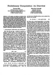
describes the application of the proposed methodology to the electric power system of Crete and presents comparative results with two other parameter identification techniques. Section V concludes the paper. II. ESTIMATION FRAMEWORK The proposed identification procedure is a simulationbased process that uses an evolutionary algorithm as optimization tool, as presented in Fig. 1. The physical system and the mathematical model of the system are excited by the same input. The output of the physical system, which is the set of available measurements, is compared to the simulated output of the model. The error between the two outputs is used as input to a genetic algorithm optimization module, which updates the model parameters in such a way that this error is minimized. r The output yˆ (t ) of the system model is a function of the system state, the input and the model parameters, as described by the set of differential-algebraic equations (1): r r r r r x& ( t ) = f ( x ( t ), z ( t ), u ( t ), a ), r r r r 0 = h ( x ( t ), z ( t ), u ( t ), a ), (1) rˆ r r r y ( t ) = g ( x ( t ), z ( t ), a ), r r X (t 0 ) = X 0 ,
r
r
where yˆ is the vector of the system model outputs, x is the r vector of the dynamical states of the system, z is the vector of r the algebraic states, u is the vector of the system inputs, and r a is the vector of the model parameters. The global state
r
[r
vector is denoted by X (t ) = x (t ) T
r z (t ) T
]
T
r
and X 0 denotes
the initial condition vector. The identification procedure estimates the unknown vector r of model parameters, a , so that the deviation between the r model and the real system responses to the same input u is minimized. The error to be minimized is the square error between the measured and the simulated output waveforms defined as (assuming discrete-time signals): T N r r 2 e(a ) = ∑∑ ( y i (t k ) − yˆ i (t k , a ) ) ,
(2)
k =1 i =1
r where y (t k ) and yˆ (t k , a ) are the measured and simulated values of the outputs at time instant t k , respectively; t k is the time sample (k = 1,..., T ) , given that T discrete observations are made on the real system, and i is the output index (i = 1,..., N ) , N being the number of outputs. The vector of
r
the unknown, constant, system parameters is denoted by a . The values of these parameters are constrained in some specific intervals. A key feature of the approach is that the estimation process is not model-specific and it is therefore straightforward to switch between a large variety of models. This advantage results from the fact that the simulation-based optimization method uses only the model output. It does not require any
knowledge of the specific model structure. The use of GAs as optimization tool enhances this feature, since one of the main features of genetic algorithms is that they do not require any auxiliary knowledge on the objective function, such as gradient information. Therefore, the proposed method is, in fact, a black-box identification method, which automatically adjusts the parameters of the model until the model output matches the measurements. r y Measured Output
Actual System
+
Test Procedures
S System Model (parameter dependent)
r yˆ
Update Parameters
Error
_ Simulated Output
Evolutionary Algorithm
Fig. 1. Block diagram of estimation procedure.
III. EVOLUTIONARY COMPUTATION TECHNIQUES FOR GENERATOR PARAMETER IDENTIFICATION A. Fundamentals of Genetic Algorithms Genetic algorithms are optimization methods inspired by natural genetics and biological evolution. They manipulate strings of data, each of which represents a possible problem solution. These strings can be binary strings, floating-point strings, or integer strings, depending on the way the problem parameters are coded into chromosomes. The strength of each chromosome is measured using fitness values, which depend only on the value of the problem objective function for the possible solution represented by the chromosome. The stronger strings are retained in the population and recombined with other strong strings to produce offspring. Weaker ones are gradually discarded from the population. The processing of strings and the evolution of the population of candidate solutions are performed based on probabilistic rules. References [18-20] provide a comprehensive description of genetic algorithms. B. Determination of Method Parameters The feasibility and adequacy of the proposed identification approach has been tested in several simple test cases with very satisfactory and promising outcomes. A number of numerical experiments were conducted, testing the effect of the various parameters of the genetic algorithm on the results. The experiments involved a single generator test system [17] and a simplified representation of an 18-machine system. In these test cases simulated waveforms were used as measurements and the estimated parameter values from the identification procedure could be directly compared to their true values. Some such preliminary results are extensively presented in [17]. The conclusions from these tests resulted in the following proposed genetic algorithm configuration.
281
C. Chromosome Representation Two types of representations have been investigated in this work, binary and real (floating-point). In floating-point representation, the chromosome is a string of real numbers, each one representing each parameter to be identified; in binary representation, each parameter is represented by a string of binary bits. Results obtained using floating-point coding were repeatedly much closer to the optimal solution compared to binary coding. Furthermore, the floating-point representation was faster and more consistent from run to run [17]. Therefore, the use of a real coded algorithm is proposed.
2) 2-point crossover, 3) Uniform crossover, 4) Arithmetical crossover. The arithmetical crossover operator creates offspring with new parameters values, defined as a linear combination of the two parents. If su and s w are to be crossed, the resulting
D. Creation of Initial Population The initial population of candidate solutions is created randomly. A population size of one to two hundred, and about one thousand generations proved to be sufficient for this problem, providing very good or even excellent results.
H. Mutation Operation In real representation, two mutation operators are implemented: uniform and non-uniform mutation. 1) Uniform mutation: This operator randomly replaces the parameter value with another one from the appropriate interval; 2) Non-Uniform mutation: This mutation type is described in [19] and it is responsible for the fine-tuning capabilities of the real-coded GA. If a parameter k of value u k of a
E. Evaluation of Candidate Solutions r Each candidate solution represents a parameter vector, a . The evaluation of each candidate solution is based on the v objective function value, e(a ) . Note that the objective function value is obtained after system simulation. The purpose of the process is to solve a minimization problem, or equivalently, a maximization problem that maximizes a transformed objective function. In this paper, the objective function to be maximized is defined as r 1 , (3) F (a ) = r e(a ) + K where K is a small positive real number used as scaling r coefficient, in order to avoid problems that may arise as e(a ) approaches zero and to control problems like premature convergence. F. Reproduction Reproduction refers to the process of selecting the best individuals of the population and copying them into a “mating pool.” These individuals form an intermediate population. Three types of the reproduction process are implemented in this work: 1) Roulette-wheel selection, 2) Tournament selection with user-defined window, 3) Deterministic sampling based on the fitness-proportionate selection scheme. No significant differences in the results were observed between the different types of reproduction in this problem. The reported results are obtained using deterministic sampling, i.e. each individual is assigned an expected number of appearances in the “mating pool,” according to its calculated fitness. Subsequently, the individuals in the “mating pool” are randomly grouped in pairs, each of which produces two offspring. G. Crossover Operation In real representation the crossover types used are: 1) 1-point crossover,
offspring are s'u = a ⋅ sw + (1− a) ⋅ su and s'w = a ⋅ su + (1− a) ⋅ sw , where a is a random number of the interval [0, 1] [19]. Uniform and two point crossover provided better results compared to other crossover types.
candidate solution is selected for mutation, its value is changed to u' k , where
⎧ u + ∆ (t , UB − u k ) u'k = ⎨ k ⎩ u k − ∆ (t , u k − LB )
(4)
depending on whether a random binary digit is 0 or 1. LB and UB are the lower and upper bounds of the interval parameter k belongs to. The function ∆(t , y ) returns a value
in the range [0, y ] such that the probability of ∆(t , y ) being close to 0 increases as the current generation number, t , increases. This property causes this operator to uniformly search the space at initial stages, when t is small, and very locally at later stages. The function used is t (1− )b
(5) ∆ (t , y ) = y ⋅ (1 − r T ) , where r is a random number in [0, 1], T is the maximal generation number, and b is a parameter determining the degree of non-uniformity [19]. In real representation, since parameters do not change during crossover, but are just recombined differently (except for the arithmetical crossover), the only way of affecting their values is by the mutation operator. So, the mutation probabilities used are increased and may reach up to 5%. The non-uniform mutation operator is vital in the performance of the algorithm when using floating-point representation. I. Creation of the Next Generation After mutation is completed, the children population is created and the previous population is replaced by the new generation. Children are evaluated and the fitness function for each individual is calculated. The procedure is repeated until the termination criterion is met, defined by a maximum number of generations. As an option, an elitist operator is also used. If this option
282
additional information for the governor-model estimation procedure, these oscillations are considered unmodeled dynamics and are treated as noise. However, no attempt was made to pre-process the measurements and eliminate this noise since it was observed in the estimation procedure results that the GA itself is able to filter out such noise very adequately. 50.00 49.95 49.90
Frequency (Hz)
is selected, the new population is not the children population, but is created by the best N individuals from the children and the previous population, where N is the population size. The aim of this elitist strategy is to eliminate the possibility of destruction of good solutions that may appear in early generations and to aid in achieving good solutions quite fast and to subsequently be able to fine-tune them. Additionally, it is expected that the best individuals will provide the best offspring after crossover. The risk of premature convergence to a sub-optimal solution is increased with this operation, but this can be controlled with the parameter K of the fitness function and with a slightly increased mutation probability.
49.85 49.80 49.75 49.70
IV. CRETE SYSTEM TEST CASE AND ESTIMATION RESULTS
49.65
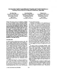
B. Transient-Response Measurements Field tests involved a conventional machine rejection under different operating conditions. Two outages were performed of 10 MW and 19 MW, at a total load of 159 MW and 208 MW, respectively. The transient behavior of the system was recorded in computers equipped with A/D converter cards. The sampling rate was 20 Hz. Recordings involved the active power response of the remaining thermal units and the system frequency deviation, which was measured at four points in the system. The total duration of each recording was 3min, including some pre-disturbance time. Data up to 10s after the disturbance were used for estimation procedure, since the dynamics of interest had reached steady state after 10s. Some typical recording are shown in Fig. 2 and 3. It is of interest to observe the active power oscillations in Fig. 3. Such oscillations of frequency around 5 Hz were observed in the output of all the diesel and steam units, even in steady-state operation. They exist because the mechanical system of the diesel units produces a pulsating torque on their shaft. The steam units are physically installed on the same power plant as the diesel units, and, therefore, they also produce a pulsating active power to compensate for the oscillations of the diesel units. Fig. 3 shows that the diesel and steam unit oscillations are in fact in opposite phase. Since modeling such oscillations would not provide any
49.60 -2.0
0.0
2.0
4.0
6.0
8.0
10.0
Time (s) 19 MW Rejection
10 MW Rejection
Fig. 2. Recordings of frequency variations of the system for the two disturbances. 15.0 14.0
Active Power (MW)
A. Test-Case System of Crete The estimation methodology has been applied to the autonomous power system of the Greek island of Crete. The power system of Crete is a relatively large, isolated system consisting mainly of oil-fired generators. It consists of 52 buses, 66 branches and 18 thermal units. Six of them are steam units, four are diesel engines, seven are gas turbines and there is a combined cycle plant. The total installed capacity is about 400MW, while the system peak load is approximately 360MW. The Greek public power corporation has conducted real time measurements of frequency and unit active power variations during intentional machine trip tests; these data were used for the identification of the governor and the unit electromechanical dynamic model parameters of each conventional generating unit.
13.0 12.0 11.0 10.0 9.0 8.0 -2.0
0.0
2.0
4.0
6.0
8.0
10.0
Time (s) Diesel Unit No 4 (MW)
Steam Unit No 3
Fig. 3. Recordings of active power variations for a stream and a diesel unit (19 MW rejection test).
C. Estimation Results The identification procedure is applied to both sets of available measurements performing two independent estimation procedures, for the different disturbances and under different loading conditions. The power system of Crete was modeled in EUROSTAG. The estimation method was implemented using the C programming language. Static network data and pre-disturbance operating conditions were provided by the electric utility, along with any available generator dynamic data. These data allowed a three-winding representation of the synchronous generators [21]. A standard IEEE Type 1 voltage regulator-exciter model was used for all units [21]. The three parameter governorturbine model shown in Fig. 4 was used. The power input of the model represents a reference command signal provided by a secondary control scheme as a power setpoint for the unit. This input was used only for units operating at constant setpoint power, and was set to zero for units operating on primary load-frequency control. Since the phenomena of interest were related only to the primary response of the units
283
10.00
no secondary control scheme was taken into consideration, as can also be concluded from the measurement duration. Σ
+ _
1 ------------TGs+1
Pmin -- Pmax Limiter
1 Pm -----------+ Tts+1 Turbine or Diesel Engine
1 ----R
Σ
1 -----------Ms+D
9.50
Active Power (MW)
Pmref.
Pe _
ωr
Rotor/Load
9.00 8.50 8.00 7.50
Governor
7.00
Fig. 4. Unit speed control and turbine (engine) dynamic model.
-2.0
Governor limits were set based on the utility provided values of minimum and maximum power output for each unit. The parameters to be identified were constrained as follows: 0.01 ≤ Ri ≤ 0.2 , 0.05 ≤ TGi ≤ 0.5s , 1 ≤ Tt steam ( j ) ≤ 3s ,
1 ≤ TDk ≤ 2s , 0.5 ≤ Tt gas ( m ) ≤ 1.5s ,
Frequency (Hz)
49.95 49.90 49.85 49.80 49.75 49.70 49.65 49.60 0.0
2.0
4.0
6.0
8.0
4.0
6.0
8.0
10.0
Recorded Active Power for Diesel 1 Unit Simulated Active Power for Diesel 1 Unit
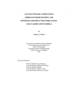
Fig. 6. Measured and simulated power output for diesel unit 1, for the 19 MW rejection test. 6.90
Active Power (MW)
6.80
each steam unit, TDk the mechanical time constant of each diesel engine, and Tt gas (m ) the turbine time constant of each
50.00
2.0
Time (s)
where Ri is the droop of each unit, TGi the governor time constant of each unit, Tt steam ( j ) the turbine time constant of
gas turbine. Results obtained after several executions of the estimation algorithm for measurements from both tests were analyzed and the final values of the unknown parameters were calculated by averaging the results, whenever some discrepancy existed. Comparative graphs of the measured transients and the simulated dynamic responses using the estimated parameters are presented in Figs. 5 through 7. The results show a considerably good agreement between the measured response and the simulated waveforms using the estimated model parameters.
0.0
6.70 6.60 6.50 6.40 6.30 6.20 6.10 -2.0
0.0
2.0
4.0
6.0
8.0
10.0
Time (s) Recorded Active Power for Steam Unit 1 Sim ulated Active Power for Steam Unit 1
Fig. 7. Measured and simulated power output for steam unit 1, for the 19 MW rejection test.
D. Comparison with Previous Estimation Approaches The same problem has been investigated using an approximate trial and error approach and a constrained optimization approach based on a modified nonlinear Simplex method. Results from these two approaches can be found in [7]. This section presents a brief comparison of these results and the results obtained by the proposed GA based identification approach. Figs. 8 through 10 indicate that the proposed approach demonstrates a more accurate performance.
10.0
50.00
Time (s)
49.95
Fig. 5. Measured and simulated system frequency for the 10 MW and 19 MW rejection tests.
49.90
Frequency (Hz)
Recorded Frequency (19 MW Rejection Test) Simulated Frequency (19 MW Rejection Test) Recorded Frequency (10 MW Rejection Test) Simulated Frequency (10 MW Rejection Test)
49.85 49.80 49.75 49.70 49.65
-2.0
49.60 -1.0 0.0
1.0
2.0
3.0
4.0
5.0
6.0
7.0
8.0
9.0
10.0
Time (s) Measured Frequency (Hz)
GA-Simulated Frequency (Hz)
Simplex-Simulated Frequency (Hz)
Trial & Error-Simulated Frequency (Hz)
Fig. 8. Comparison of simulated and measured waveforms of frequency, for parameter values from different estimation procedures (19 MW rejection test).
284
[3]
10.50
Active Power (MW)
10.00
[4] 9.50 9.00
[5]
8.50
[6]
8.00 -2.0
-1.0
0.0
1.0
2.0
3.0
4.0
5.0
6.0
7.0
8.0
9.0
10.0
Time (s) Diesel Unit 4 Measured
Diesel Unit 4 GA-Simulated
Diesel Unit 4 Simplex-Simulated
Diesel Unit 4 Trial & Error-Simulated
[7]
Fig. 9. Comparison of simulated and measured waveforms of active power of diesel unit 4, for parameter values from different estimation procedures (19 MW rejection test). 38.00
[8]
Active Power (MW)
37.00
[9]
36.00 35.00
[10]
34.00 33.00
-2.0
32.00 -1.0 0.0
[11] 1.0
2.0
3.0
4.0
5.0
6.0
7.0
8.0
9.0
10.0
Time (s)
[12]
Gas Turbine 6 Measured
Gas Turbine 6 GA-Simulated
Gas Turbine 6 Simplex-Simulated
Gas Turbine 6 Trial & Error-Simulated
Fig. 10. Comparison of simulated and measured waveforms of active power of gas unit 6, for parameter values from different estimation procedures (19 MW rejection test).
[13] [14]
V. CONCLUSION This paper investigates the application of evolutionary computation techniques for the identification of governorturbine dynamic models. The paper proposes the use of a realcoded genetic algorithm as optimization tool for the estimation procedure. The main advantages of the proposed methodology are its accuracy, the few input data required, its flexibility, and the simplicity of its mechanism. However, its main drawback is the execution speed, mainly due to the large number of simulations involved. The proposed method has been successfully applied to the simultaneous identification of the turbine–governor models of the units of the medium size, isolated power system of Crete. Comparison with the results obtained from other methods shows the superiority of the proposed GA approach.
[2]
[16]
[17]
[18] [19] [20] [21]
REFERENCES [1]
[15]
M. Shen, V. Venkatasubramanian, N. Abi-Samra, and D. Sobajic, “A new framework for estimation of generator dynamic parameters,” IEEE Trans. Power Systems, vol. 15, no 2, pp. 756–763, May 2000. T. Inoue, H. Taniguchi, Y. Ikeguchi, and K. Yoshida, “Estimation of power system inertia constant and capacity of spinning reserve support generators using measured frequency transients,” IEEE Trans. Power Systems, vol. 12, no 1, pp. 136–142, February 1997.
285
D. J. Trudnowski and J. C. Agee, “Identifying a hydraulic–turbine model from measured field data,” IEEE Trans. Energy Conversion, vol. 10, no 4, pp. 768–773, December 1995. Z. Zhao, F. Zheng, J. Gao, and L. Xu, “A dynamic on–line parameter identification and full–scale system experimental verification for large synchronous machines,” IEEE Trans. Energy Conversion, vol. 10, no 3, pp. 392–398, September 1995. L. N. Hannett and A. H. Khan, “Combustion turbine dynamic model validation from tests,” IEEE Trans. Power Systems, vol. 8, no 1, pp. 152–158, February 1993. N. D. Hatziargyriou, E. S. Karapidakis, and D. Hatzifotis, “Frequency stability of power systems in large islands with high wind power penetration,” in Proc. 1998 Int. Conf. Bulk Power System Dynamics and Control IV–Restructuring, August 24–28, 1998, Santorini, Greece, pp. 699–704. N. D. Hatziargyriou, G. S. Stavrakakis, E. S. Karapidakis, F. Dimopoulos, and K. Kalaitzakis, “Identification of synchronous machine parameters using constrained optimization,” in Proc. 2001 Power Tech Conf. (PowerTech ’01), vol. 4, September 10-13, 2001, Porto, Portugal. P. Pillay, R. Nolan, and T. Haque, “Application of genetic algorithms to motor parameter determination for transient torque calculations,” IEEE Trans. Industry Applications, vol. 33, no 5, pp. 1273–1282, Sep/Oct 1997. P. Nangsue, P. Pillay, and S. E. Conry, “Evolutionary algorithms for induction motor parameter determination,” IEEE Trans. Energy Conversion, vol. 14, no 3, pp. 447–453, September 1999. J. R. Smith, F. Fatehi, C. S. Woods, J. F. Hauer, D. J. Trudnowski, “Transfer function identification in power system applications,” IEEE Trans. Power Systems, vol. 8, no 3, pp 1282-1290, Aug, 1993. J. C. Wang, H. D. Chiang, C. T. Huang, Y. T. Chen, C. L. Chang, C. Y. Huang, “Identification of excitation system models based on on-line digital measurements,” IEEE Trans. Power Systems, vol. 10, no 3, pp.1286-1293, Aug. 1995. C. P. Cheng, C. W. Liu, and C. C. Liu, “Unit commitment by lagrangian relaxation and genetic algorithms,” IEEE Trans. Power Systems, vol. 15, no 2, pp. 756–763, May 2000. I. G. Damousis, A. G. Bakirtzis, and P. S. Dokopoulos, “Networkconstraint economic dispatch using real-coded genetic algorithm,” IEEE Trans. Power Systems, vol. 18, no 1, pp. 198–205, February 2003. E. L. da Silva, H. A. Gil, and J. M. Areiza, “Transmission network expansion planning under an improved genetic algorithm,” Proc. 21st Int. Conf. Power Industry Computer Applications (P.I.C.A.), May 16-21, 1999, Santa Clara, CA, U.S.A., pp. 315–321. M. M. Begovic, B. Radibratovic, and F. C. Lambert, “On multiobjective volt-VAR optimization in power systems,” in Proc. 37th Annual Hawaii Int. Conference on System Sciences, Hawaii, January 5-8, 2004, pp. 5964. D. Srinivasan, F. Wen, C. S. Chang, and A. C. Liew, “A survey of applications of evolutionary computing to power systems,” Proc. Int. Conf. Intelligent Systems Applications to Power Systems (I.S.A.P.), January 28-February 2, 1996, Orlando, FL, U.S.A., pp. 35–41. G. K. Stefopoulos, N. D. Hatziargyriou, and P. S. Georgilakis, “Identification of governor-turbine parameters using evolutionary computation,” Proc. Int. Conf. Intelligent Systems Applications to Power Systems (I.S.A.P.), June 17-21, 2001, Budapest, Hungary, pp. 288-293. D. E. Goldberg, Genetic Algorithms in Search, Optimization, and Machine Learning. Reading, MA: Addison-Wesley, 1989. Z. Michalewicz, Genetic Algorithms + Data Structures = Evolution Programs. New York: Springer-Verlag, 1996. Z. Michalewicz and D. B. Fogel, How to Solve It: Modern Heuristics. New York: Springer-Verlag, 1999. P. Kundur, Power System Stability and Control. New York: McGrawHill, 1994.