We present an algorithm called the exact ceiling point algorithm (XCPA) for solving the pure, general integer linear programming problem (P). A recent report by ...
An Exact Ceiling Point Algorithm for General Integer Linear Programming Robert M. Saltzman School of Business, San Francisco State University, San Francisco, California 94132 Frederick S . Hillier Department of Operations Research , Stanford University, Stanford, California 94305
We present an algorithm called the exact ceiling point algorithm (XCPA) for solving the pure, general integer linear programming problem (P). A recent report by the authors demonstrates that, if the set of feasible integer solutions for (P) is nonempty and bounded, all optimal solutions for (P) are “feasible l-ceiling points,” roughly, feasible integer solutions lying on or near the boundary of the feasible region for the LP-relaxation associated with (P). Consequently, the XCPA solves (P) by implicitly enumerating only feasible l-ceiling points, making use of conditional bounds and “double backtracking.” We discuss the results of computational testing on a set of 48 problems taken from the literature.
1. INTRODUCTION This article describes an algorithm called the exact ceiling point algorithm (XCPA) for solving the pure, general integer linear programming problem whose form is Maximize cTx = z subject to Ax
5
b
x 2 0, x integer,
(PI
where A E 6 E A‘“,and c E :‘R”. We assume that the data are rational but unrestricted in sign. For ease of exposition, we further assume that A and c are integer. An important additional assumption is that no implicit or explicit equality constraints are used to define the feasible region FR = { x 2 0 I Ax 5 b } for (LP), the linear programming relaxation associated with (P). For a discussion of applications of (P), see [12, 221. The XCPA was developed to systematically search for feasible “l-ceiling points” first introduced in [18]. An integer solution x is a l-ceiling point with Naval Research Logistics, Vol. 38, pp. 53-69 (1991) CCC 0028-1441/91/080053-17%04.00 Copyright 0 1991 by John Wiley & Sons, Inc.
54
Naval Research Logistics, Vol. 38 (1991)
respect to the ith constraint, abbreviated “x is a l-CP(i),” if (1) x satisfies afx 5 b,, where a, is the ith row of the constraint matrix A , and (2) modifying some component of x by + 1 or - 1 yields a solution which violates this constraint, i.e., for some j , a,’x + Iu,,~ > b,. Thus, if x is a 1-CP(i) then x narrowly satisfies the ith constraint: Taking a unit step from x toward the ith constraint hyperplane in a direction parallel to some coordinate axis results in an infeasible point. Similarly, an integer solution x is defined to be a l-ceiling point with respect to the feasible region FR, abbreviated ‘ ‘ x is a l-CP(FR),” if (1) x E FR and (2) modifying some component of x by 1 or - 1 leads to a solution which violates one or more constraints, i.e., for some j , 3 i: afx + la,,\ > b,. Note that x is a 1-CP(FR) if and only if x is a feasible 1-CP(i) for some (i). Theorem 2 of [18] demonstrates that, if the set of feasible integer solutions for (P) is nonempty and bounded, all optimal solutions for (P) are 1-CP(FR)’s. Consequently, one way to solve (P) is to enumerate its 1-CP(FR)’s. The general framework of the XCPA follows that of the bound-and-scan algorithm (BASA) due to Hillier [15], although the two algorithms differ in many important details. Both the XCPA and the BASA first call upon a heuristic algorithm to find an initial solution whose objective function value is then used to define a search region S. In addition, both are incumbent-improving algorithms which implicitly enumerate solutions within S by using conditional variable bounds. However, the XCPA differs from the BASA and all other algorithms in that its seeks only l-CP(FR)’s within S. In enumerating solutions, the XCPA employs conditional bounds similar to those derived by Krolak [16], but the process of updating these bounds is new, as is a way of fathoming large numbers of solutions which we call “double backtracking.” Another distinguishing feature of the XCPA is its novel application of an “intersection cut” introduced by Balas [ 5 ]t o define a region which is searched initially in order to speed up the XCPA. Intially, the XCPA executes the heuristic ceiling point algorithm (HCPA) [ 191, which includes solving (LP), so Section 2 states the assumptions needed for these steps and describes how S is constructed. Section 3 discusses how the search within S is limited by seeking l-ceiling points with respect to one specific constraint. The restricted region, called a search hyperrectangle, is defined by a set of unconditional variable bounds. The process of enumerating l-ceiling points within a search hyperrectangle is described in Section 4 and put into perspective in Section 5 , which gives an overview of the entire algorithm. Section 6 discusses the preliminary search made with respect to an intersection cut. We report our computational experience in Section 7 and conclude in Section 8.
+
2. ASSUMPTIONS As in [15], we assume that the set of feasible solutions for (LP) is nonempty and bounded, and that there is a unique optimal solution X for (LP) which is not all integer. The implications of these assumptions are examined in [15]. The XCPA begins by finding X , the set of constraints binding at X,and the set of K extreme directions emanating from X (so K = n barring degeneracy), which The XCPA also asumes an initial feasible integer solution form the cone x H , with objective function value z , is provided by the HCPA. We first establish a region S which must be searched either to find an optimal
m.
Saltzman and Hillier: Integer Programming
55
solution for (P) or to verify that x H is optimal. For k = 1, . . . , K , let p L be the point of intersection between the kth extreme direction emanating from X and the objective function hyperplane cTx = z , and, for notational convenience, let p o = X. Under the above assumptions,-all optimal solutions for (P) are contained in the convex hull S of the (K + 1) extreme points {PO, p ’ , . . . ,p ” } , as implied by Theorem 1 in [15]. Thus, we may confine our search to S without fear of missing any optimal solutions for (P). Nonbinding constraints which do not intersect S,for instance, may be dropped from further consideration. We seek solutions which are strictly better than x H so actually use the objective function hyperplane cTx = z + 1 in the determination of the p k ’ s .Lower and upper bounds [ S , for each variable x , can be found by taking the minimum and maximum, dspectively ,over the jth component of all vertices of the resulting S and rounding appropriately. For j = 1, . . . , n, the bounds
s,]
S, = max{[min{pf}l, 0},
-
k
-
S, = Imax{pf}],
where [ 1 and 1 1 denote rounding up and rounding down, respectively, define what we shall refer to as SHR(S), the search hyperrectangle for S . (Cabot and Erenguc [9] also define an initial hyperrectangle in their branch-and-bound algorithm for integer separable programming, but continually break it down into smaller and smaller hyperrectangles during their branching procedure by imposing Dakin constraints.) Whenever a new incumbent solution is found, SHR(S) is recomputed with respect to a new objective function hyperplane. If S, > 3, for any j , then SHR(S) = 0; the problem is solved since there are no feasible integer solutions better than the incumbent. Otherwise, we begin to search for 1-CP(FR)’s.
3. UNCONDITIONAL VARIABLE BOUNDS The major distinction of the XCPA is that it seeks only feasible l-CP(i)’s and does so with respect to one “search constraint” at a time. One consequence of this approach is that we further restrict our attention to a subhyperrectangle of SHR(S) which depends upon the choice of the search constraint (i). This search hyperrectangle, denoted SHR(i), is contained within SHR(S) but is still large enough to contain all feasible l-CP(i)’s better than the incumbent. A second Consequence is that we impose an additional constraint based on part (2) of the definition of 1-CP(i). An integer solution x is a 1-CP(i) if it satisfies both (i) a,’x 5 b, and (i’) a,’x 2 b, - t , , where f, = max, - 1. For example, all feasible 1-CP(1)’s better than the incumbent lie in the darkly shaded region of Figure 1. The search region SHR( 1) is constructed using (l), (1’), and S,as we now describe. First, let El be the set of extreme rays emanating from X which lie on the ith constraint hyperplane. Also, let q k be the point of intersection between the kth extreme ray of FR and the translated constraint hyperplane (i‘), for all k q! E,. For instance, the point q2 in Figure 1 is the intersection of constraint hyperplane (1‘) and extreme ray 2, where extreme ray 2 coincides with constraint hyperplane (2). The search hyperrectangle associated with the ith constraint, SHR(i), is
IU, ~
56
Naval Research Logistics, Vol. 38 (1991)
Figure 1. Feasible 1-CP(1)'s better than the incumbent lie in the darkly shaded region.
defined by the ranges {[l,., u,], j = 1, . . . , n } , where the bounds for x, are formed by taking the minlmum and maximum, respectively, over the jth component of all points defining the hyperrectangle and rounding appropriately. Furthermore, these bounds need be no wider than those defining SHR(S): 1, = max{~min{min{p,k},Xi, min{q,k}}l, Sj> kEE,
keE,
and
If I, 3 ui for any j , then there are no integer solutions in SHR(i), and a new search constraint is identified. Assuming this is not the case, we proceed to enumerate the integer solutions contained within SHR(i). 4. ENUMERATING SOLUTIONS WITHIN THE SEARCH HYPERRECTANGLE
Once SHR(1') has been constructed, finding l-CP(i)'s better than the incumbept amounts to examining SHR(i) for solutions which are feasible with respect to all the relevant constraints, including (i'). Since SHR(i) G SHR(S), any feasible solution found will become the new incumbent. When this occurs, the intersection points between the extreme rays emanating from X and the new objective function hyperplane move closer to X. With a smaller set S , the bounds defining SHR(S) may tighten. If so, the unconditional variable bounds developed for the current search constraint will also tighten, possibly leading to tighter conditional variable bounds as well. Thus, as we backtrack from a new incumbent solution, the conditional bounds are recomputed. The enumeration process is
Saltzman and Hillier: Integer Programming
57
ill -
Next value o f X J
XI
i
XI
AX1
t Calcul ate/Upaale condltlonsl bobnas
IL). U l l o n X I
no
x)
= F i r s t value
- AX1
v
t
Figure 2. Flow diagram of the XCPA's enumeration scheme
shown as a flow diagram in Figure 2. Two features which differentiate it from a simple exhuastive enumeration scheme, namely, the use of conditional variable bounds and the potential for "double backtracking," are described i n the next two subsections.
4.1. Conditional Variable Bounds In a manner similar to Balas' for the binary case [4], one can also erlumerate general integer solutions by specifying the values of individual variables one at x., . . . . x , - I ) . a time. Furthermore. given the values of the fixed variables (s,. one can develop conditional bounds [ L , Ix, I . U,1 x,..,] for the variable xi. (In Figure 2 these conditional bounds are abbreviated as [ L , , U , ] . )This approach has been taken before for the general integer case. Hillier [15] develops 4 different bounding procedures for four different groups of variables by using the extreme points of S and weights associated with them. Our approach is similar to that of Krolak [16], who works directly with the constraints of the problem. After introducing some notation. we briefly review this approach since we wish to extend the work of [16].
Naval Research Logistics, Vol. 38 (1991)
58
First, let
be the gap or slack remaining in constraint (i) after having fixed xl, . . . , Also, let
be the minimum amount of the gap g j j that may be used up by fixing variables , . . . , x, within their unconditional bounds. Feasibility of a complete solution x with respect to the ith constraint requires
x, +
Let Ljjlxj-, and Ujjlxj-ldenote the lower and upper conditional bounds, respectively, on xi when constraint (i) is considered alone after fixing x l , . . . , xi-1.Then (1) implies Lijlx,-l
{ (gjj i,,
-
w j . j + l ) / u j j 7 if aii < 0 if ajj 1 0
and
The desired conditional lower and upper bounds Ljlxi-l and U ~ X ~on- xi ~ ]must maintain feasibility with respect to all constraints and therefore are
and
The bounds (2) and (3) are very similar to those defined by Krolak [16]. If we find L,lx,-, > U,(x,-, for any j , then there are no feasible completions of the partial solution (xl, . . . , x / - ~ and ) we backtrack to the next value of x,-~. At first glance, it may appear that calculating L,llx,-l and Uf,lx,-l each time xJ-l changes is computationally prohibitive, but actually it is not. Krolak did not recognize that both Lf/lxJ-,and U f ~ l x , -change l in a predictable way as x / - ~ changes. Both are linear functions with a slope that can be calculated once at
59
Saltzman and Hillier: Integer Programming
the outset of the algorithm. To see this, let u,-] be the current value of x , - ~and U I - ~the value to which it is then changed, so u ; - ~= u,-] + d,-l, where d,-] E { - 1, +1}. Let L , , I X ~and - ~ U,,[X;-~ denote the lower and upper conditional bounds, respectively, on x, when considering constraint (i) alone after fixing variables (x,, . . . , x , - ~ ,x , - ] ) to ( u , , . . . , u , - ~ u, ; - ~ ) .Similarly, let g,,l~,-~ denote the quantity g,, given the partial solution ( u l , . . . , u,-2, U , - J and g,,lx;-l the quantity g,, given the partial solution ( u , , . . . , u , - ~ u, ; - J . When a,, > 0, we are interested in how U , , ~ X differs , - ~ from U , , ~ X - ~ :
U,,Ix;-l
- fL/IX,-l
=
[(g,,lx;-l
-
K./+J-
(E?1,IX/-l
- W,~,+l)l~~I/
,,,-
where f,, = a /a,,- Since both f,, and d,_l are independent of the value of x,- U , , ~ X ,is- ~a linear function of x,_ with slope 5 f l , . When a,,< 0, a similar ~ a linear functon of x , - ~with slope kf,,. derivation reveals that L , , ~ Xis, -also Therefore, after calculating U,,lx,-l and L , , ~ Xfor ,-~ the initial value of x , - ~ ,one of the conditional bounds aIways changes in an additive fashion while the other remains equal to the value of its unconditional bound:
and
4.2.
Doable Backtracking
In addition to being easy to update, L , , ~ X and , - ~ U,,~X,-~ impart an important property to the conditional bounds L, Ix,- and 17I , x, - As the maximum over a set of linear functions, L,lx,-, is a convex functon of x , - ~by a well-known , -the ~ minitheorem (see [3, Theorem 4.131, for example). Similarly, U , ~ X is mum over a set of linear functions and therefore a concave function of This is illustrated in Figure 3 for the case in which a,, 2 0, for all (i, j ) , so that L,Ix,-, = I,. As x , _ ] ranges between its conditional bounds L,-llx,-2 and U,-llx,-z, the - ~ U , ~ X ,may _ ~ ,cross once, twice or not at conditional bounds on x,, L , ~ X ,and all. If we observe that L , ~ X ,exceeds -~ U,~X,-~ for a particular value of x , - ~ ,we can certainly backtrack to x;-~, the next value of x , - ~ ,because there are no feasible completions of the partial solution (x,, . . . , x,-,). However, it is also for all remaining values of x , - ~due to possible that L,lx,_, will exceed U,IX,_~ the convexity and concavity properties of the conditional bounds. In this case, we can double backtrack, i.e., backtrack to the next value ofx,-z. The following
Naval Research Logistics, Vol. 38 (1991)
60
Figure 3. Upper and lower conditional bounds on x , when all a,, 2 0.
theorem gives a condition for when it is possible to double backtrack, thereby significantly reducing the amount of enumeration.
,
,
THEOREM 1: Suppose the backtracking condition L, I x, - > U, Ix,- holds for a particular value of x , - ~ . A sufficient condition to double backtrack, i.e., skip all remaining integer values of x , - ~within its conditional bounds, is that -f,s,-, 2 -fs,6,-1, for some r such that Lr, = max,{L,,(~,-~} and some s such that Us, = minf{Uf,lx,-l}. PROOF:
L,)X;-~ 2 L,lx,_, - fr,d,-l,
where r is such that L ,
=
max(L,,Ix,-,) I
> U,I x , - ~ - f r,6j-,,
z U,lx,-,
-
fS,d,-,,
by the backtracking condition where s is such that Us,= min(U,,(x,-l} I
Repeating the argument €or subsequent values of x, - 1, we find that the lower conditional bound on r, exceeds the corresponding upper cwditional bound for all remaining values of x , - ~within its conditional bounds. Thus, we can double backtrack. 0 Constraint indices r an# s are readily available, having been identified in the calculation of L, 1 x , - ~and U, I x,- 1, respectively. We only check the double backtracking condition after we have found that we can perform any ordinary back-
Saltzman and Hillier: Integer Programming
61
tracking step. The condition of Theorem 1 must be checked due to the possibility that the conditional bounds may cross twice as x, moves between its conditional bounds. If we double backtracked after the first observation of the lower conditional bound exceeding the upper conditional bound, we could miss some partial solutions with feasible completions. Double backtracking seems to be most helpful on problems in which the unconditional bounds are fairly wide for one or more variables, such as the fixed-charge problems reported on in Section 7. ~
5. OVERVIEW OF THE EXACT CEILING POINT ALGORITHM Figure 4 shows how the process of enumerating 1-ceiling points with respect to a single constraint fits into the XCPA. (Step 2 is described in Section 6.) The iterative part of the XCPA, Step 3, essentially “branches” on a functional constraint (i) and seeks to “fathom” subregion SHR(1’) of SHR(S) by enumerating all of its feasible 1-CP(i)’s. Suppose that the best feasible solution known after having searched SHR(i) is xi with objective function value z = cTxi.If a new set S’ is formed by the objective function hyperplane cTx = z + 1 and the constraints binding at X, then S’ excludes the best-known solution x i . It is possible that S’ contains no integer solutions and the problem has been solved. If this is not the case, we replace the previous search constraint (i) by the translated constraint (i”) a,’x Ibi - maxilaiiI. This yields a modified problem (P’) which remains to be searched. The modified relaxation, (LP’), is then solved for its optimal solution and value (X’,2’). Note that 2’ < 2 = cT1 and that 5‘ is an upper bound on the optimal objective function value for (P‘). Therefore, if 2’ Iz, the problem is solved with x i as an optimal solution for (P). If the problem 2not solved, a new iteration begins by selecting another search constraint. The criterion for selecting a new search constraint favors constraints which, upon being fathomed, guarantee a large reduction in the new upper bound 7 .To summarize, the XCPA proceeds in a “search and cut” fashion until the problem is solved. (See [20] for further details about the algorithm.)
STEP 0: (a) Solve ( L P ) j (T, Z = c 5 ) . (b) Apply heuristic ceiling point algorithm (HCPA) j (x,,,z = crx,,). STEP 1: Construct S and search hyperrectangle S H R ( S ) . STEP 2: (a) Construct intersection cut ( I ) and search hyperrectangle SHR(Z). (b) Enumerate feasible l-CP(I)’s within S H R ( I ) 3 ( x , , ~= crx,). (c) Stop if g = f ;otherwise, STEP3: REPEAT (a) Select a search constraint ( i ) and construct SHR(1’). (b) Enumerate feasible 1-CP(i)’s 3 (x,,g = cTxx,). (c) Replace (i) aTx 5 b, with (i”) aTx I b, - max, lu8,1. (d) Resolve (LP’)to obtain ( T ’ , f ‘ = cry’). UNTIL OPTIMAL (SHR(S)= 0 or 1 2 T’).
Figure 4. Outline of the exact ceiling point algorithm (XCPA).
62
Naval Research Logistics, Vol. 38 (1991)
THEOREM 2. Suppose the set of feasible solutions for (P) is nonempty and bounded, X is unique and z > --. Then the iterative procedure of the XCPA (Step 3 of Figure 4) is guaranteed to find an optimal solution for (P) in a finite number of steps. PROOF: Based on [18, Theorem 21 and [15, Theorem 13, the total region T which must be searched to solve the problem is that portion of S containing 1-CP(FR)’s:
Since T consists only of subsets of S, T is bounded. Also, there are only a finite number of constraints, each of which is searched at most once for its 1-ceiling points. What remains to be shown is that the scheme of Section 4 for enumerating 1-ceiling points with respect to a specific constraint is finite. For a given constraint (i), a search hyperrectangle SHR(i) is defined and then examined for 1-CP(i)’s. Being a subset of T , SHR(i) is bounded, i.e., all unconditional bounds {[f,, u,], j = 1, . . . , n} are bounded. The conditional bounds {[L,lx,-1, U, IX,-~], j = 1, . . . , n} are also bounded since, by construction, L,!x,, 2 f,and U,lx,- 5 u, for all j . Thus, the total number of integer solutions contained within SHR(i) is finite. Finally, the scheme which enumerates integer solutions within SHR(i) examines at most once each complete solution or partial solution leading to one or more complete solutions. A partial solution is fathomed if it is shown to be unable to lead to a feasible completion which is better than the incumbent. A completed solution is fathomed by virtue of becoming the new incumbent. Thus, the scheme of Section 4 is finite. 0
6. SEARCHING THE INTERSECTION CUT After the heuristic ceiling point algorithm has run, but prior to searching any original constraint for its 1-ceiling points, a preliminary search is made for the 1-ceiling points with respect to a specially constructed constraint called an intersection cut. Intersection cuts were developed in [5, 61 as a class of cutting planes for solving integer programming problems. They possess the usual feature of chopping off X without eliminating any feasible integer solutions for (P). They also happen to require the same structural information from the (LP) as does the XCPA. Our interest in these cuts stems not from their ability to solve (P) as part of an iterative cutting plane procedure, but from their ability to define a region near X which is likely to contain a near-optimal feasible integer solution. Searching for 1-ceiling points with respect to the intersection cut (I) is similar to the procedure used for an original functional constraint (i) described earlier in that a search hyperrectangle SHR(I) is first defined and then searched for 1CP(Z)’s. The only difference is that our SHR(Z) is not so large as to contain all of the 1-ceiling points with respect to (I), but only some of them. A nice feature about the intersection cut is that the volume of SHR(1) reflects the shape of the feasible region near X. When the cone FR is narrow, the SHR(Z) is apt to contain a relatively small number of integer solutions and so not much time will
Saltzman and Hillier: Integer Programming
63
be wasted
searching an unpromising region. On the other hand, when the cone FR is fairly wide, SHR(1) is apt to contain a relatively large number of integer solutions and the subsequent search will be thorough in a part of the feasible region with a good chance of containing an optimal solution. 7. COMPUTATIONAL RESULTS
The XCPA was tested on a DEC VaxStation I1 with 10 megabytes of main memory, under the MicroVMS operating system, version 4.5. The algorithm was coded in Fortran (see [20] for a listing) and compiled with the VAX Fortran Compiler, version 4.5, using the default settings that include an optimizer. All execution times are in CPU seconds; those that apply specifically to the XCPA include the time required to read in the data but not to write out any information. To assess the effectiveness of the XCPA, we compared its performance to those of other algorithms on 48 test problems taken from the literature. It should be emphasized that these results provide only a general indication of an algorithm’s performance rather than conclusive evidence, because not only are we examining performance based on a relatively limited amount of computational experience, but also the algorithms have been coded by different authors, run on computers of different generations and sizes, etc. The test problems have been grouped into two categories: “realistic” (because these problems were drawn from real applications) and “randomly generated” (because the parameters of these problems were randomly generated). All 24 of the realistic problems appeared in the study by Trauth and Woolsey [23]. These consist of ten “fixed-charge” problems, {FC-1, . . . , FC-lo}, five “setcovering” problems, {IBM-1, . . . , IBM-5}, and nine “allocation” problems, {AL-55, AL-60, . . . , AL-100). Though small, the FC and IBM problems are hard to solve because the optimal solutions for (P) and (LP) are relatively far apart. Characteristic of the FC problems is that simple rounding of X almost never yields a feasible integer solution. The AL problems are all the same single constraint 0-1 knapsack problem, except that b, increases from 55 to 100. With one exception, all 24 randomly generated problems are due to Hillier [15]. These problems, labeled {I-1, 1-2, 1-5, I-6}, {11-1, . . . , 11-14} and (111-2, . . . , 111-5, 111-8}, all have at least 15 variables and 15 constraints. Their integer coefficients were generated from a uniform distribution over various intervals (see [15, Table I]). The one additional problem, labeled “11-M,” was solved in [17] and is similar to a Type I1 problem. With constraint matrices which are essentially 100 percent dense, general integer variables, and large b,’s, the Type I and Type I1 problems are relatively difficult to solve. The Type I11 problems are 0-1 problems that are less challenging. For algorithms which also solve the LP relaxation, one performance measure is the ratio of total CPU time to CPU time required to solve (LP). This ratio gives an idea of how much work is required by the entire algorithm relative to an efficient and dependable algorithm (the simplex method) used in the first phase of the algorithm to solve (LP). It also provides a crude basis of comparison for LP-based algorithms which perhaps have been coded in different languages and/or tested on different computers. With this measure, the execution times of various algorithms’ are normalized by the amount of time to solve (LP). Note,
64
Naval Research Logistics, Vol. 38 (1991)
however, that the LP solvers embedded within the respective integer programming algorithms may have been designed and implemented quite differently, causing such comparisons to be rather rough. Table 1 shows the performance of the four phases of the XCPA on the test problems. The first four columns, respectively, give the fraction of the total CPU time spent solving (LP), running Phases 2 and 3 of the heuristic ceiling point algorithm (HCPA) , searching the intersection cut, and executing the iterative portion of the XCPA. The next-to-last column gives the total CPU time in seconds, while the last column gives the ratio of the total CPU time to the amount of time spent solving (LP). Based on both total CPU time and the ratio of total CPU time to time spent solving (LP), the XCPA appears to efficiently solve all of the realistic problems except IBM-5. Excluding IBM-5, the only realistic problems where the bulk of the CPU time was spent on Step 3 of the XCPA were {FC-5, . . . , FC-8). These four problems are poorly scaled versions of {FC-1, . . . , FC-4}, i.e., some of the b,’s were increased by a factor of 10, greatly enlarging the feasible region. To solve each of these problems, all constraints binding at X had to be searched for 1-ceiling points. Searching the intersection cut proved ineffective on all of the fixed-charge problems (except FC-lo), another indication of their difficulty. The XCPA’s performance on the randomly generated problems varied with the problem type. This is partly because the same is true of the HCPA, which provides the XCPA with an initial feasible solution x H . The better the objective function value of x H , the smaller S is, and hence, the quicker the XCPA solves (P). On all five Type I11 problems, the HCPA identified an optimal solution and the XCPA verified its optimality rather quickly. Of the 15 Type I1 problems, the HCPA located an optimal solution in six cases. On the remaining nine Type I1 problems, searching the intersection cut was effective in locating a better solution four times, one of which was optimal. While only moderately successful, the intersection cut search is cheap enough computationally to make it worthwhile. The iterative step of the XCPA was successful in solving the majority of Type I1 problems fairly quickly. However, it was slow in finishing off 11-8 and 11-12 and failed to prove optimality on 11-13, 1-5, and 1-6 within the allocated time (15 minutes). In Tables 2 and 3, the XCPA is compared with other exact algorithms, one of which is part of a widely available package called the Generalized Algebraic Modeling System (GAMS, Version 2.04) developed by Brooke, Kendrick, and Meeraus [8]. When faced with a mixed integer linear programming problem, GAMS calls upon the Zero/One Optimization Methods (ZOOM/XMP, Version 2.0). In brief, ZOOM converts every general integer variable into a sum of binary variables, applies the Pivot & Complement heuristic device of Balas and Martin [7] to find an initial solution, and proceeds with an LP-based branchand-bound scheme. Tight upper bounds were specified in order to keep the number of binary variables small and are listed in Appendix A of [20]. A blank table entry indicates that no time was reported for that algorithm on that problem. Only the XCPA and GAMS/ZOOM were executed on the same computer, so it is difficult to directly compare all of the stated execution times. However, based on one study of various computers’ performances [lo], a knowledgeable computer scientist [21] informed us that the IBM-370/168 may be as
Saltzman and Hillier: Integer Programming
65
Table 1. Execution times of the exact ceiling Doint algorithm. % of total CPU time
Problem
LP
Heuristic
FC-1 FC-2 FC-3 FC-4 FC-5 FC-6 FC-7 FC-8 FC-9 FC-10
50.0 69.6 56.5 76.5 22.1 25.4 21.7 27.3 51.5 25.0
25.0 26.1 13.0 17.6 23.5 23.7 25.0 25.4 15.1 51.7
IBM-1 IBM-2 IBM-3 IBM-4 IBM-5
53.8 55.0 60.0 24.2 1.3
28.2 40.0 28.0 75.8 4.1
AL-55 AL-60 AL-65 AL-70 AL-75 AL-80 AL-85 AL-90 AL-100
27.5 51.8 41.1 43.3 100.0 39.7 39.5 38.9 100.0
72.5 28.6 46.6 56.7 0.0 45.2 44.7 47.2 0.0
1-1 1-2 1-5 1-6 11-1 11-2 11-3 11-4 11-5 11-6 11-7 11-8 11-9 11-10 11-11 11-12 11-13 11-14 11-M 111-2 111-3 111-4 111-5 111-8
0.1 1.1 2000 >1837 4.8 4.6 13.6 9.7 3.5 66.3 54.3 252.7 4.5 11.1 8.8 308.7 >1154 37.2 45.3 2.8 3.4 4.9 2.5 2.6
66
Naval Research Logistics, Vol. 38 (1991)
Table 2. Comparison of performances by exact algorithms on realistic problems. GAMSI Accelerated 1ip-1 XCPA ZOOM BASA [I1] SCPA [2] [13] VaxStation I1 VaxStation I1 IBM-360167 370/168 7090 Problem Time Ratioa Time Ratioa Time Ratio8 Time Time 10.7 0.19 1.83 4.30 2.0 14.8 0.32 FC-1 0.28 9.0 1.4 11.6 0.27 0.19 1.35 FC-2 0.23 3.13 3.41 11.4 0.33 11.0 FC-3 0.23 0.13 1.88 1.8 0.13 1.48 2.24 1.3 7.7 0.28 9.3 FC-4 0.17 0.18 9.01 464.4 8.62 4.5 27.8 41.77 FC-5 0.68 0.18 7.57 220.7 FC-6 0.59 12.68 3.9 39.6 22.07 8.22 4.6 24.9 41.77 1392.3 0.09 7.83 FC-7 0.60 12.05 38.9 21.81 0.09 6.42 727.0 FC-8 0.55 3.7 1.92 7.2 0.40 3.23 1.9 5.6 0.43 FC-9 0.33 1.61 9.15 13.67 4.0 14.9 FC-10 1.16 3.02 1.9 6.9 0.53 1.87 6.6 IBM-1 0.39 6.46 15.4 0.55 3.02 6.9 IBM-2 0.40 1.8 1.7 11.8 0.21 10.5 IBM-3 0.25 3.19 2.87 33.97 4.1 22.8 11.67 IBM-4 2.69 77.2 >671 9.28 15.5 IBM-5 47.10 >900 66.48 AL-55 1.09 1.04 3.6 2.7 0.18 2.42 AL-60 0.56 1.9 1.04 2.7 0.19 5.08 AL-65 0.73 2.4 3.0 1.26 0.14 3.90 AL-70 0.67 2.3 3.2 1.27 0.18 2.60 AL-75 0.28 1.0 1.0 0.34 0.15 1.87 2.5 AL-80 0.73 2.8 1.02 0.15 3.87 2.5 AL-85 0.76 3.2 1.33 0.17 7.88 AL-90 0.72 2.6 3.9 1.22 0.16 4.52 1.0 1.0 AL-100 0.29 0.31 0.17 1.87 “Ratio = Total CPU time/CPU time solving (LP).
much as five times faster than the IBM-360167 and seven times faster than the VaxStation 11. For the realistic problems, Table 2 compares the XCPA, GAMSIZOOM, the accelerated bound-and-scan algorithm of Faaland and Hillier’s [ 111 run on an IBM-360/67, the surrogate cutting plane algorithm (SCPA) of Austin and Ghandforoush’s [2] (an extension of their reduced advanced start algorithm [l] run on an IBM-370/168, and the cutting plane code LIP-1 of Haldi and Isaacson [13] run on an IBM-7090. Based on the execution times and relative speeds of the computers, the XCPA appears to be highly competitive with each of the other algorithms on all of the realistic problems except IBM-5. For the randomly generated problems, Table 3 compares the XCPA, GAMS/ ZOOM, Hillier’s bound-and-scan algorithm (BASA) [15] run on an IBM-360/ 67 and the SCPA. The total time figures for the BASA were compiled by adding the times for the heuristic algorithm described in [14] to those times given in [15], since the best solution yielded by the heuristic algorithm was used as an initial solution for the BASA [15, p. 6681. Overall, both the SCPA and the BASA appear to be faster and more consistent than the XCPA and GAMS/ ZOOM on problems of Type I and 11. While the XCPA is competitive with these two algorithms on about half of the Type I1 problems, GAMS/ZOOM is
Saltzman and Hillier: Integer Programming
67
Table 3. Comparison of exact algorithms on randomly generated problems.
Problem
XCPA VaxStation I1 Time Ratio"
1-1 1-2 1-5 1-6
348.49 40.37 >900 >900
645.4 85.9 >2000 >1837
11-1 11-2 11-3 11-4 11-5
2.13 2.08 6.79 3.99 1.44
4.8 4.6 13.6 9.7 3.5
11-6 11-7 11-8 11-9 11-10
28.49 23.35 116.26 2.09 4.98
66.3 54.3 252.7 4.5 11.1
11-11 11-12 11-13 11-14 11-M
6.17 231.50 >900 30.48 13.13
8.8 308.7 >1154 37.2 45.3
111-2
1.37 1.52 1.85 1.00 0.94
2.8 3.4 4.9 2.5 2.6
111-3
111-4 111-5
111-8 "Ratio
=
GAMWZOOM VaxStation I1 Time Ratioa 429.96 462.3 407.84 261.4 >900 >612 >900 >967 83.48 132.5 64.92 95.5 79.34 90.2 83.32 119.0 59.30 76.0 78.39 137.5 74.97 88.2 93.45 118.3 47.83 83.9 97.58 112.2
4.40 2.65 3.89 6.50 5.92
6.7 4.1 7.8 11.4 9.6
BASA [15] 1BM-360'67
Time
SCPA [2] IBM-370/ 168
Ratioa
Time
17.32 2.94 19.49 9.34
19.0 3.2 20.5 7.5
3.18 1.10
2.68 2.33 2.21 2.28 1.48
3.9 2.9 3.8 3.2 2.4
0.92 0.98 1.20 1.02 0.81
3.30 3.22 4.22 1.85 2.53
5.4 5.4 6.2 2.9 3.1
1.16 1.90 1.93 0.68 0.85
6.48 7.17 162.25 7.38
2.0 2.1 144.9 6.7
1.32 1.61 1.60 1.58 1.41
2.4 2.5 2.7 2.8 2.3
0.40 0.55 0.52 0.39 0.45
Total CPU time/CPU time solving (LP).
not really competitive at all. On Type I11 problems, the XCPA, the BASA, and the SCPA all appear to be of roughly comparable efficiency. Even on the 0-1 problems (classes AL and Type 111) for which it was designed, GAMYZOOM did not perform as well as the XCPA, which is not designed for 0-1 problems.
8. SUMMARY The exact ceiling point algorithm is based upon theorems indicating that (P) may be solved by enumerating only the 1-CP(FR)'s lying within the set S . The algorithm systematically searches for feasible 1-CP(i)'s with respect to one constraint at a time. While enumerating such solutions, conditional variable bounds and double backtracking are used to accelerate the fathoming process. Because the iterative part of the XCPA benefits greatly by having a good initial solution, a preliminary heuristic search is made for 1-ceiling points with respect to an intersection cut, thereby examining a promising part of the feasible region first. Our computational experience leads us to believe that the XCPA is a good approach for tackling some problems, but not the best approach for tackling others. Specifically, the XCPA performs very well on the set of realistic problems, but not as well as two other algorithms on some of the more difficult randomly
68
Naval Research Logistics, Vol. 38 (1991)
generated problems. On the set of realistic problems, particularly the fixedcharge problems, the double backtracking feature seems to be very helpful in quickly fathoming large numbers of solutions. However, this feature seems to be of little help on the randomly generated problems because there is no pattern to the ratios from one column to the next. Also, when the HCPA did not find a very good solution, as was the case for most of the Type I problems, it often led t o an inefficient performance by the XCPA. Further research is needed to determine what types of problems are best suited t o our ceiling point approach.
REFERENCES Austin, L. and Ghandforoush, P., “An Advanced Dual Algorithm with Constraint Relaxation for All-Integer Programming,” Naval Research Logistics Quarterly, 30, 133-143 (1983). Austin, L. and Ghandforoush, P., “A Surrogate Cutting Plane Algorithm for AllInteger Programming,” Computers & Operations Research, 12, 241-250 (1985). Avriel, M.,Nonlinear Programming: Analysis and Methods, Prentice-Hall, Englewood Cliffs, NJ, 1976. Balas, E., “An Additive Algorithm for Solving Linear Programs with Zero-One Variables,” Operations Research, 13, 517-546 (1965). Balas, E., “Intersection Cuts-A New Type of Cutting Planes for Integer Programming,” Operations Research, 19, 19-39 (1971). Balas, E., Bowman, V., Glover F., and Sommer, D., “An Intersection Cut From the Dual of the Unit Hypercube,” Operations Research, 19, 40-44 (1971). Balas, E. and C. Martin, “Pivot and Complement: A Heuristic for 0-1 Programming,” Management Science, 26, 86-96 (1980). Brooke, A., D. Kendrick, and A. Meeraus, GAMS: A User’s Guide, The Scientific Press, Redwood City, CA, 1988. Cabot, A. and S. Erenguc, “A Branch and Bound Algorithm for Solving a Class of Nonlinear Integer Programming Problems,” Naval Research Logistics Quarterly, 33, 559-567 (1986). Dongarra, J . , “Performance of Various Computers Using Standard Linear Equations Software in a Fortran Environment,” ACM SIGNUM Newsletter, 19,23-26 (1984). Faaland, B. and Hillier, F., “The Accelerated Bound-and-Scan Algorithm for Integer Programming,” Operations Research, 23, 406-425 (1975). Garfinkel, R. and G. Nemhauser, Integer Programming, John Wiley, New York, 1972. Haldi, J., and Issacson, L., “A Computer Code for Integer Solutions to Linear Programs,” Operations Research, 13, 946-959 (1965). Hillier, F., “Efficient Heuristic Procedures for Integer Linear Programming with an Interior,”Operations Research, 17, 600-637 (1969). Hillier, F., “A Bound-and-Scan Algorithm for Pure Integer Linear Programming with General Variables,” Operations Research, 17, 638-679 (1969). Krolak, P., “Computational Results of an Integer Programming Algorithm,” Operations Research, 17, 743-749 (1969). Land, A. and A. Doig, “An Automatic Method of Solving Discrete Programming Problems,” Econometrica, 28, 497-520 (1960). Saltzman, R., and F. Hillier, “The Role of Ceiling Points in General Integer Linear Programming,’’ Technical Report No. SOL 88-11, Department of Operations Research, Stanford University, Stanford, CA, 1988. Saltzman, R. and F. Hillier, “A Heuristic Ceiling Point Algorithm for General Integer Linear Programming,” Technical Report No. SOL 88-19, Department of Operations Research, Stanford University, Stanford, CA, 1988. Saltzman, R., and F. Hillier, “An Exact Ceiling Point Algorithm for General Integer
Saltzman and Hillier: Integer Programming
69
Linear Programming,” Technical Report No. SOL 88-20, Department of Operations Research, Stanford University, Stanford, CA, 1988. [21] Saunders, M.,private communication, November 3, 1988. [22] Taha, H . , Integer Programming: Theory, Applications and Computations, Academic Press, New York, 1975. [23] Trauth, C. and R. Woolsey, “Integer Linear Programming: A Study in Computational Efficiency,” Management Science, 15, 481-493 (1969).