Feb 23, 2011 - changes in field theory, which often proceeds via nucleat- ing a bubble of true vacuum inside a sea of false vacuum by a quantum mechanical ...
DESY 11-028
An Exact Tunneling Solution in a Simple Realistic Landscape Koushik Dutta, Pascal M. Vaudrevange, and Alexander Westphal Deutsches Elektronen-Synchrotron DESY, Theory Group, D-22603 Hamburg, Germany (Dated: February 23, 2011)
arXiv:1102.4742v1 [hep-th] 23 Feb 2011
We present an analytical solution for the tunneling process in a piecewise linear and quadratic potential which does not make use of the thin-wall approximation. A quadratic potential allows for smooth attachment of various slopes exiting into the final minimum of a realistic potential. Our tunneling solution thus serves as a realistic approximation to situations such as populating a landscape of slow-roll inflationary regions by tunneling, and it is valid for all regimes of the barrier parameters. We shortly comment on the inclusion of gravity.
Vacuum decay is one of the most drastic environmental changes in field theory, which often proceeds via nucleating a bubble of true vacuum inside a sea of false vacuum by a quantum mechanical tunneling event. Tunneling processes (in first order phase transitions) play a vital role in many aspects of high-energy theory and cosmology. The groundwork for the computation of tunneling amplitudes was laid many years ago by Coleman and de Luccia (CdL) [1, 2]. Their method uses the Euclidean path integral to calculate what is now known as the CdL instanton, often appearing to be the stationary point of minimal action. The CdL analysis consist of a single real scalar field in a potential with a false and a true vacuum located at the position of the corresponding minima of the scalar potential, φ+ and φ− respectively, see Figure 1. The tunneling probability per unit volume Γ/V = Ae−B , can be conveniently expressed [12] in terms of the Euclidean action SE of the O(4) symmetric so-called bounce solution φBounce as B = SE [φBounce ] − SE [φ+ ] . In the interior of the nucleating bubble, the scalar field exits at some point on the slope towards the minimum, while outside of the bubble, beyond the bubble wall, it still sits in the false minimum. In general, the equation of motion for the bounce is difficult to solve analytically. This lead to the development of the thin-wall approximation [1]. In this limit of small energy difference between the true and false vacuum, the bubble wall becomes infinitely thin, and an approximate solution can be found. To the best of our knowledge, an exact tunneling solution is only known in the case of a piecewise linear potential [3]. In this article, we will derive the analytic tunneling solution for the piecewise linear and quadratic potential � VL ≡ λ+ φ + V− + 12 m2 φ2− , φ < 0 , (1) V (φ) = VR ≡ 12 m2 (φ − φ− )2 + V− , φ ≥ 0 (see Fig 1) which does not make use of the thin-wall approximation, see also recent work by [4]. However, one (non-differential) equation remains to be solved either numerically or in the limits of a large and small bubble radius. We show that our general analytical results reduce to the thin-wall results and the results of [3] in the appropriate limits. For the most part of this work, we exclude the effects of gravity and thus ignore the magnitude
of the true vacuum energy V− . We will only offer some qualitative arguments about the inclusion of gravity in the end, except for the thin-wall limit. We expect this tunneling solution to be the simplest yet realistic approximation to an arbitrarily shaped barrier exiting smoothly into a true minimum. The reason is that a quadratic potential towards the true vacuum allows us to attach to its critical point smoothly a given shallowly sloped region of scalar potential containing a minimum. This may be particularly relevant for studying the dynamics of populating a landscape of slow-roll inflationary slopes via tunneling from some false vacuum. Any discussion of the relative prevalence of different classes of inflationary models in a candidate fundamental theory such as string theory will necessarily have to include the discussion of the bias incurred by population via tunneling. In the absence of gravity, the Euclidean action for a single scalar field with potential energy V (φ) is given by � � Z ∞ 1 02 2 3 SE = 2π dr r φ + V (φ) , (2) 2 0 and the bounce solution φ(r) is determined by solving the Euclidean O(4) symmetric equations of motion 3 (3) φ00 (r) + φ0 (r) = ∂φ V , r where φ0 ≡ ∂r φ and the potential for our case is given by Eq. (1). Initially, the field is sitting in the false vacuum at φ+ < 0, kept in place by a linear potential piece (shown as a dashed line in Fig 1) attached to the left of the false minimum. Its slope is irrelevant in the following computation as long as it classically stabilizes the field in the false minimum. To start with, we first depict the numerically solved bounce solution schematically in Fig 2. The field sits at some value φ0 (not necessarily close to the true vacuum φ− = 1 in this case but to the right of the maximum of the potential) inside the bubble at r = 0. At the bubble radius RT , the field crosses through the maximum of the potential at φ(RT ) = 0. Well outside the bubble, the field sits in the false vacuum φ(R+ ) = φ+ = −0.0001. The solutions φL and φR in the left and right part of the potential, respectively, have to fulfill the following boundary conditions: The bubble nucleates at rest
2
VT
to obtain B =
2π 2 φ2− RT2 [α2 −
V+
V-
0
Φ+
Φ-
4 √ I2 (mRT ) α ∆+ 3 I1 (mRT )
(1 − ∆) 2 2 m RT ], 8
√ 2α +
� mRT (7)
0 Φ+ RT
R+
FIG. 2: The bounce solution for α = 10−5 , ∆ = 10−5 , m = 10−6 , φ− = 1.The field sits at some value φ = φ0 = 0.0037 inside the bubble at r = 0. At the bubble radius, the field crosses through the maximum locus of the potential at φ(RT ) = 0. Well outside the bubble, the field sits in the false vacuum φ(R+ ) = φ+ = −0.0001. For the definitions of α, ∆ see the text below Eq. (7).
φR (0) = φ0 > 0, φ0R (0) = 0 . Outside of the bubble wall at finite r > R+ , the field sits at rest in the false vacuum i.e φL (R+ ) = φ+ , φ0L (R+ ) = 0. Solving Eq. (3) with these boundary conditions for both parts of the potential, we find � λ+ 2 2 , = φ+ + 2 r 2 − R + 8r I1 (mr) = φ− + 2(φ0 − φ− ) , mr
∆mRT = mRT
I2 (mRT ) , I1 (mRT )
(8)
which can be solved numerically. However, it is much more instructive to examine it in the limits of large and small mRT . But first we should briefly note that Eq. (8) can be used to remove the Bessel functions from Eq. (7). We emphasize that the above expression for B now depends on the potential parameters and the only unknown quantity RT , which is fully determined in terms of α, ∆ by an algebraic Eq. (8). This is one of our central results. Now we turn towards the two approximate solutions of our results. We start by taking the limit mRT � 1, and in this limit, Eq. (8) can be solved as
Φ0
φL
�
where we have introduced α = −φ+ /φ− > 0, and ∆ = (−2λ+ φ+ )/(m2 φ2− ) as a measure of the height of the potential barrier with values 0 < ∆ < 1. In order to find RT , we combine Eq. (6) to get
FIG. 1: Schematic shape of the potential Eq. (1)
0
1 + 2
(4)
mRT =
3 + 4α 1 √ . 2 1− ∆
(9)
We note that for all allowed values of α and ∆, mRT > 23 . In particular, we find that mRT can be large either for the thin-wall limit ∆ ≈ 1, or ∆ < 1, but α > ∆ (see Eq. (20)). For the latter case, the potential minima are separated by sizable distances in the field space, as well as the potential energy between the false and true vacuum. Therefore, the large mRT limit encompasses more than the just thin-wall solution, see Table I. For small differences in the vacuum energy � = (1 − ∆) 12 m2 φ2− , in leading order of �, mRT ≈
(3 + 4α)m2 φ2− , 2�
(10)
where I1 (z) is the modified Bessel function of the first kind (see also equation (3.14) in [1]). In order to determine the constants φ0 , R+ , and RT , we use that the field configurations need to match smoothly at the bubble radius RT with φL (RT ) = φR (RT ) = 0 and φ0L (RT ) = φ0R (RT ). Thus we need to solve
which we will find to be identical to the result from using the thin-wall formalism. This is in accord with expectations from the thin-wall formalism: The radius of the nucleating bubble grows toward ∞ as the minima become degenerate. Also, looking at the limit of the matching condition φR = 0 in Eq. (6) r � � π φ0 = φ− 1 − (mRT )3/2 e−mRT , (11) 2
8RT2 φ+ φ− mRT , I1 (mRT ) = , λ+ 2(φ− − φ0 ) 8RT2 = (φ− − φ0 )I2 (mRT ) . (6) λ+
it is clear that the true vacuum bubble nucleates close to the minimum of the quadratic part of the potential, φ0 ∼ φ− , for large values of mRT . Plugging in the expression for RT from Eq. (9) yields an unwieldy result for B. Thus we only display the expression for B in the � → 0 limit
φR
(5)
2 (R+ − RT2 )2 = − 4 R+ − RT4
Calculating the Euclidean action Eq. (2) for the solutions Eq. (4), we can express both φ0 and R+ in terms of RT
B ≈
π2 4 8 4 m φ− (3 + 4α) . 96�3
(12)
3 Finally, we give an expression of B in terms of φ0 B ≈
� π 2 φ2− φ0 � 3 (4α + 3) · ln 1 − . 12m2 φ−
(13)
In summary, in this limit, when either the thin-wall approximations are valid or the minima are separated far away from each other, a large bubble nucleates close to the true vacuum. For the sake of comparison, we shall now give the essential results of the thin-wall calculation, where the nu27π 2 S 4 cleation rate is given by B = 2�3 1 and for the potential Eq. (1) we can compute S1 directly, and in the small � limit it is � � m 4 S1 = − 1 + α φ2− . (14) 2 3 Plugging this into the expression for B we find the same expression as Eq. (12). The same way, we get RT = 3S1 /� which, after plugging in S1 and expanding in �, agrees with (10). We will now proceed to the opposite case of taking the limit of small mRT � 1. To second order in mRT , Eq. (8) is solved by �√ � √ mRT = 2 ∆ + 2α + ∆ , (15) where we discarded the negative solution. Now mRT < µT can be equivalently casted as (0 < α < µ2T /8) ∧ (0 < ∆ < (µ2T − 8α)2 /16µ2T . Therefore small mRT limit corresponds to the small values of α and ∆, where potential minima are closely spaced in the field space, but the potential difference between the false and the true minima is considerably large. In this limit, the exit point of the bubble can be conveniently expressed as � φ0 = φ− 1 +
8 mRT
�−1 ,
(16)
and it shows that the bubble nucleates close to the tip of potential barrier which is intuitively understandable from the form the potential in this particular limit. We can express B for small mRT in terms of α, ∆ as B =
16π 2 φ2− (2α + ∆) 3" m2
(17) !# r � � 2α 2α × (α + ∆)2 + ∆2 1 + 1+ 1+ . ∆ ∆
Again, we give an expression of B in terms of φ0 " √ � �3/2 � �2 # 16π 2 φ2− φ 4α 2∆ φ φ 0 0 0 B≈ α2 + +∆ (18) m2 φ− 3 φ− φ− In the limit where the quadratic part of the potential can be regarded as almost flat, the solution we found for small mRT should agree with the results of a piecewise
mRT α = 0.01 0.6 α = 0.1 1.2 α = 0.5 2.5
Bexact 0.0023 0.3 23.9
BDJ 0.0022 0.04 0.6
Bthin−wall 72.4 113.3 529.8
TABLE I: The mismatch of action: the linearized result BDJ of [3] compared to the thin-wall result Bthin−wall and the exact result found here. B is given in units of φ2− /m2 and all values are quoted for ∆ = 0.01. Clearly, there are regimes with mRT = O(1) where neither the linearized treatment of [3] nor the thin-wall approximation are sufficient.
linear potential as studied by [3]. This is the case for the limit ∆ � 1. Taking the slope of the quadratic potential to be λ− = m2 φ− , the parameter c defined by [3] becomes c = 2α/∆. The value of the tunneling radius mRT found by [3] is given by mRT = √
4α √ 2α + ∆ − ∆
(19)
in agreement with the corresponding expansion of Eq. (15). Expanding the expression for B in Eq. (7), we find perfect agreement with B from [3]. Let us recall what has been done so far. We reduced the computation of the tunneling amplitude for tunneling from the linear to the quadratic part of the potential Eq. (1) to solving an exact Eq. (8). We provided approximate solutions for the limits of large and small tunnel radius mRTL,S . Surprisingly, the smaller of the relative error between either the numerical result RTN and RTL or RTS is always smaller than 10%, see Fig. 3 (a). This then defines globally the approximate solution mRT √ � q � 2α 2 2 ∆ 1 + 1 + ∆ , ∆ < (0.8α − 0.5) (20) mRT = 1√ 3+4α 2 , (0.8α − 0.5) < ∆ 2
1− ∆
In other words, we succeeded in computing the tunneling amplitude analytically in a non thin-wall solution with error better than 50%, see Fig. 3 (b). Finally we shall comment on the effects of gravity on the tunneling process. In the thin-wall limit [2] studied the case where either true or false vacuum are at zero energy, whereas [5] examined this issue for arbitrary values of the false and true vacuum energy. Among other things, their work suggests the following intuitive idea. When the true vacuum is also in de-Sitter space, due to the “pull” on the bubble both from the inside and the outside of the wall, the nucleation rate should be enhanced compared to the flat space limit. We can see this explicitly in the thin-wall approximation, i.e. large mRT and 1 − ∆ � 1, where the effect of gravity is well understood. Following [5], we compute the effect of gravity on the exponent B of the tunnel rate, see Fig. 3 (c). For sufficiently sub-Planckian values of φ− we always have a constant asymptotic value for B/B0 , where B0 is without gravity. In the case of small η− ≡ m2 /V−
4
10 0.1
0.3
0.3
0.2
0.2
0.1
0.1
0.0
0.0
0.8 0.0
a)
α 0.6
0.0
0.4 ∆
0.4
0.8
0.2 1.0 0.0
0.001 B 10-5 B0 10-7
b)
0.2
α 0.6
0.4 ∆ 0.8
0.2 1.0
Α = 0.1 Α=1
Η- 10
3
Η- 1
10-11 10-4 0.001 0.01
0.6 0.4
Η- 106
10-9
0.8
0.6 0.2
∆B /B
0.5 0.4
∆RT /RT
0.5 0.4
c)
Η- 10-3 0.1 Φ-
1
10
100
FIG. 3: The smaller of the relative error between the numerical value of RT (panel a) and B (panel b) and its small or large mRT limit, Min(|RTN − RTL |/RTN , |RTN − RTS |/RTN ). The relative error is always smaller than 10% for RT and 50% for B. c) B/B0 of the tunneling rate for ∆ = 0.95 in the presence of gravity as a function of φ− , with η− ≡ m2 /V− .
(i.e a very flat quadratic part) the ratio B/B0 is very small, giving a large gravitational enhancement of tunneling. Contrary, for a steep potential with large η− the tunneling probability is less enhanced. Increasing α suppresses B further and thus enhances tunneling. This fits with the notion, that the gravitational correction is more important the thicker the barrier is in the field space, since for a given φ− the barrier thickness increases with increasing α. Note, that for α � 1 and η− � 1 there is also Hawking-Moss tunneling possible [6–8]. In this work we have discussed quantum tunneling in field theory in a piecewise linear and quadratic scalar potential with a a false vacuum and a true vacuum. Such a potential is arguably the most simple yet realistic approximation to an arbitrarily shaped barrier exiting smoothly into a true minimum. The reason is that a quadratic potential allows us to attach to its critical point smoothly a given shallowly sloped region of scalar potential containing a minimum. Our result gives the tunneling rate in this situation exactly. Further, in the appropriate limits our result reduces to either the thin-wall result or the known result for piecewise linear potentials by [3]. However, there is a large region of barrier shape parameter space where neither of them is a good approximation to the full solution given here. The inclusion of further effects from approximating a given potential to higher
than quadratic order, as well as a detailed incorporation of gravity in the non-thin-wall regime we leave as a topic for future work. Let us note in passing that in the context of meta-stable supersymmetry breaking vacua in gauge theories [9], choosing Nf = 3Nc /2 flavors can imply a barrier shape with α � ∆ ' 2/3. For α = 0.1 this gives mRT ' 9 which shows the linearized result of [3] with BDJ ' 2.5 × 10² overestimating the tunneling rate by an order of magnitude compared to our exact result B ' 1.4 × 10³ . Finally, we expect one relevant application of our results to be the dynamics of populating a landscape of slow-roll inflationary slopes via tunneling from some false vacuum. For this purpose, we have given the instanton action for the tunneling also as a function of φ0 , as the exit from the tunneling φ = φ0 , φ˙ 0 = 0 forms the initial conditions for slow-roll inflation.
[1] S. R. Coleman, Phys. Rev. D15, 2929 (1977). [2] S. R. Coleman and F. De Luccia, Phys. Rev. D21, 3305 (1980). [3] M. J. Duncan and L. G. Jensen, Phys. Lett. B291, 109 (1992). [4] U. Gen and M. Sasaki, Phys.Rev. D61, 103508 (2000), arXiv:gr-qc/9912096 [gr-qc] . [5] S. J. Parke, Phys.Lett. B121, 313 (1983). [6] A. D. Linde, Nucl. Phys. B372, 421 (1992), arXiv:hepth/9110037 . [7] S. W. Hawking and I. G. Moss, Phys. Lett. B110, 35 (1982).
[8] A. A. Starobinsky, In *De Vega, H.j. ( Ed.), Sanchez, N. ( Ed.): Field Theory, Quantum Gravity and Strings*, 107-126. [9] K. A. Intriligator, N. Seiberg, and D. Shih, JHEP 04, 021 (2006), arXiv:hep-th/0602239 . [10] G. Pastras, (2011), arXiv:1102.4567 [hep-th] . [11] C. G. Callan Jr. and S. R. Coleman, Phys. Rev. D16, 1762 (1977). [12] A is of order m4 with m being the characteristic scale of the problem [11], which we neglect here for simplicity.
Note added: While this paper was being finished, we became aware of [10], which overlaps with our results. Acknowledgements: We are grateful to A. Linde for enlightening comments. This work was supported by the Impuls und Vernetzungsfond of the Helmholtz Association of German Research Centres under grant HZ-NG603, and German Science Foundation (DFG) within the Collaborative Research Center 676 Particles, Strings and the Early Universe.