Mar 12, 2014 - a moon bound rocket using variable-structure to in- crease the simulation .... framework is implemented in Python and allows a user to define a ...
An example of beneficial use of variable-structure modeling to enhance an existing rocket model Alexandra Mehlhase Daniel Gomez Esperon Julien Bergmann Marcel Merkle Technical University of Berlin, Department of Software Engineering Ernst-Reuter-Platz 7, 10587 Berlin
Abstract This paper introduces a rocket model and discusses the advantages of refining it using a variable-structure approach to remodel critical parts. Both versions of the model are implemented in Modelica and were simulated using Dymola as simulation environment. The DySMo framework, which supports the simulation of variable-structure models in common simulation environments, was used to facilitate the redesign. The general benefits of the variable-structure approach are presented, and on the basis of the rocket model we present that simulation time and the data volume of the simulation can be reduced while maintaining the accuracy of the simulation results. variable-structure modeling, simulation speed, data reduction, reduce equation stiffness, rocket launch
1
Introduction
In this paper, we regard the benefits of modeling a moon bound rocket using variable-structure to increase the simulation speed and to reduce the amount of saved simulation data. The aim of our simulation is to predict the trajectory of the rocket, beginning with the ignition on earth’s surface up until it reaches the moon as destination. The rocket is multi-staged, and as such consists of three booster modules and a payload module without means of propulsion. The model takes into account the chemical reactions in the boosters combustion chambers, which generate the thrust, the gravity of both earth and moon as well as atmospheric influences. First, we introduce a classical implementation of the model, which we will then compare to a redesigned version that uses the variable-structure approach. The classical model calculates all components during the entire simulation. However the time frame DOI 10.3384/ECP14096707
of the chemical reactions and of the rocket’s movement are very different, which results in a stiff system of equations. This stiff equation system necessitates small step sizes, although a great part of the equation set would permit rather large time steps. Additionally, the chemical reactions only need to be calculated as long as the thrust of the rocket has not reached a steady state. As a result, the simulation of the classical model generates an exceeding overhead of unnecessary simulation data and calculations. The ability to enable and disable equations during runtime, holding certain values constant for a given period of time, would allow to reduce this overhead. However, Modelica requires a constant set of equations and does not allow to change the equation system while simulating. All equations have to be solved during the whole simulation. In special cases and with the use of some workarounds the equation system can be manipulated to a certain degree, but not in the extend we want to use in this paper. In section 2, we introduce the concept of variablestructure models and discuss different approaches to implement and simulate them. We will then give a detailed overview over the rocket model as well as the redesigned version in section 3. We compare the simulation results of both models, regarding performance and accuracy as well as the volume of generated data, in section 4.
2
Variable-Structure Modeling
The aim of variable-structure modeling is to improve models by introducing the means to change their equation and variable set during simulation. This is realized by encapsulating certain sets of equations and variables into different models, to which we refer as modes, and implementing a way to switch between them. Each transition is triggered by a predefined
Proceedings of the 10th International ModelicaConference March 10-12, 2014, Lund, Sweden
707
An example of beneficial use of variable-structure modeling to enhance an existing rocket model
switching condition. The mode switch is then realized by storing the end values of certain variables and using them to initialize variables of the next mode. The decision, which end values are used to initialize variables of the subsequent mode, has to be made by the modeler. Variable-structure models are the topic of numerous publications, although they are often referred to by different names. In [6, 8] they are introduced as ’Multimodels’, whereas they are referred to as ’Structurally dynamic systems’ in [4] and ’Variable structure systems’ in [10]. As they feature discrete mode switches as well as continuous equation systems they are often considered a variant of hybrid systems. A noteworthy method of formally specifying hybrid systems is the DEVS formalism, introduced in [9, 7]. Currently, altering the set of equations at runtime is not easily achieved using common Modelica simulation environments, which we want to use for the rocket simulation. However, several approaches to introduce variable-structure to a Modelica model have been devised, an overview is given in [1]. One way is presented in [2], where conditional statements are used to enable and disable certain equations based on disjunct conditions, which distinguish the current mode of the model. Such an approach is classified as Maximal state space, as the models state space is static and holds all states regardless of the current mode. This may lead to complicated mode switching procedures, as more than just the equations relevant at the current time have to be taken into account. Additionally, it may prove difficult to add new modes to an existing model. We followed another approach, termed Hybrid decomposition, where each mode is implemented as a separate model and the simulation switches between these models based on switching conditions. Mosilab [5] and SOL [10] are two approaches which enable the user to create variable-structure models. But since they are based on own languages it would be necessary to re-implement the rocket model in the specific language. In our approach we want to use common simulation environments. A framework to use common simulation environments is DySMo [3]. This framework is implemented in Python and allows a user to define a variable-structure model. The framework then handles the switches between the different modes automatically. In this framework Simulink, Dymola and OpenModelica are integrated. The communication with the tools is based on a communication interface integrated in Python. New interfaces can easily be added to the framework and then be used as simulation 708
environments for the variable-structure model. A basic overview of the sequence used in the framework for switching between different modes is illustrated in Figure 1. Each of the gray boxes is a method defined in the communication interface from the specific simulation environment for the currently active mode. As a first step, all modes are compiled, which is necessary for the Modelica simulation environments. When all modes are compiled, the simulation parameters (determining start time, stop time, solver, etc.) are set in the framework. Mode Control Compile modes
Write init file Simulate
Update mode
Read endvalues
Input/Output mapping
Read observer
Find transition
t < stop time Save observer
Figure 1: Schematic view of the steps to simulate a variable-structure model in DySMo After this initial setup, the simulation of the first mode, using the appropriate executable and initialization file, is started. Each mode contains a certain number of stop conditions, which define when a simulation is terminated. When such a stop condition is reached, a variable switch_to is set, which indicates the next mode of the simulation. Then the simulation terminates. The framework now reads the simulation results of the recently terminated simulation, and maps those endvalues to the starting values of the variables of the subsequent mode. Finally, the mode is updated to the new mode and a new simulation is started. When the final stop time of the simulation is reached, the simulation terminates and the saved sim-
Proceedings of the 10th International ModelicaConference March 10-12, 2014, Lund, Sweden
DOI 10.3384/ECP14096707
Session 4E: Hybrid Systems
ulation data is stored in a file. Using DySMo allows us to introduce variable structure to an existing model without having to completely re-model it, as only minor changes have to be made to add the stop conditions and make the desired adjustments to the equation sets of each mode. Furthermore, in certain modes we are able to greatly reduce the state space to only hold the needed information. This approach shown here is of course only suitable and sensible for models with a small number of modes. If many mode switches occur this framework is not suitable and in the future, creating and simulating variablestructure models should be integrated into Modelica or other languages. But since this is not the case yet, we want to illustrate the positive effects these kinds of models have with the DySMo prototype.
3
Rocket Model
In this section we introduce the classical as well as the redesigned model in greater detail. Both models were implemented in Modelica and simulated using Dymola. The object-oriented, component-based nature of Modelica allowed us to separate our model into different components which facilitated the variablestructure redesign.
important physical laws necessary to create the rocket model. As the main interest was the trajectory of the rocket, we needed Newton’s law of motion F (s,t) = Fprop + Fg − Fd = m · s. ¨ The remaining task was to determine F. In our model the force consists of three parts. The aerodynamic drag (Fd ), the gravitational force (Fg ) and the propulsive power (Fprop ). The gravitation force is dependent on the planets (Earth and Moon) and their masses. Also the position and mass of the rocket have an influence. The aeoredynamic drag is essentially 1 Fd = cW ρAv2 2 and is only calculated while the rocket is still in the atmosphere of the earth. The remaining force is calculated by simulating the combustion of hydrogen in the combustion chamber. Therefore many thermodynamical and chemical laws come into play. We will mention only a few. It is possible to model the change of concentration during a chemical reaction A+E → D+F
Earth Fg Fd near earth ⇒ Fd 6= 0 f ar f rom earth ⇒ Fd = 0
with ordinary differential equations C˙A = −kCACE , C˙D = kCACE etc.
Fg_earth , Fd
Rocket body movement speed direction
Fprop , m
Propulsion stage chemical reactions create thrust start of stage ⇒ Fprop 6= 0 steady state ⇒ Fprop = const empty fuel ⇒ Fprop = 0
Fg_moon
where k = BT
nf
� � E exp − . RT
Moreover we assume the ideal gas law
Moon gravitational force (Fg ) orientation point
p=n
RT . V
It is then possible to determine the temperature using Figure 2: Components of the rocket model and properties that are calculated by them
Basic mathematical description of the rocket Since the complete Model consists of many equations, it would be too long to explain all equations in detail. However we give a short overview about the most DOI 10.3384/ECP14096707
ρcv
r dT = ∑ (−∆uk ) wk dt k=1
plus vaporization and heating terms. Here ∆uk is the reaction energy of reaction k. For a chemical reaction i where two substances A and B react, the coefficient wi is defined as wi := kiCACB . This energy leads to pressure which leads to a massflow through a thottle with
Proceedings of the 10th International ModelicaConference March 10-12, 2014, Lund, Sweden
709
An example of beneficial use of variable-structure modeling to enhance an existing rocket model
a certain velocity. At the end the propulsive power can propulsion stage accurately, even though the propulsion is no longer needed after a steady state is reached be calculated with or once the rocket runs out of fuel. As each simulaFprop = mv. ˙ tion step generates data for all variables of the model, The original and the variable-strucutre model were the overall data volume of a simulation measures about separated into different components, namely the 1.5GB and postprocessing this data becomes rather terocket body, the propulsion stage and two celestial dious work. bodies, as shown in Figure 2. The figure already gives a short overview of what different calculations are nec- 3.2 Variable-structure Redesign essary in each component. When introducing variable structure to a model, the first step is always to identify the modes that are to 3.1 Original Model be implemented, or, to put it another way, to deterBasically, the rocket body calculates the movement of mine in which way the model could benefit from varithe rocket by taking into account the forces it is ex- able structure. As already discussed, the rocket model posed to. The propulsion stage is responsible to cal- has a stiff equation set, which necessitates very small culate the thrust the rocket produces. It contains three step sizes for the simulation to be reasonably accubooster modules that are used in succession. Each of rate. However, only during the ignition of each booster the booster modules has a specified amount of fuel module it is necessary to calculate the chemical reacavailable and calculates the chemical reactions for the tions inside the combustion chamber with such accucombustion of the solid propellant. This combus- racy. Afterwards, the thrust is almost constant and retion builds up a pressure in the combustion chamber, garding the chemical reactions is not necessary anythrough which the thrust of the rocket is determined. more. Furthermore, the rocket has to travel a great distance After starting a new stage the thrust is build up quite fast and afterwards is almost constant. These chemical without any thrust at all to reach the moon. The result reactions necessitate the solver to employ very small is that the simulation runs with a very small step size step sizes, as they take place very rapidly. Whenever for a long time while the variables feature only minithe fuel of a booster module runs out, the propulsion mal changes. The aim of our redesign is to eliminate this problem stage will reinitialize using the next booster module available. Once the last booster module is emptied, by holding the thrust constant once it has fully build up and take the equations for the chemical equations the rocket will no longer generate thrust. The celestial bodies are used to represent the moon out of the model. After fuel runs out, the rocket either and the earth. They supply the gravitational forces in- switches to another booster and builds up the thrust fluencing the rocket. Air resistance and wind are also anew (regarding the chemical reactions), or it switches calculated in the earth component, as the rocket is sub- to a mode where thrust is assumed as zero if no further jected to these while passing through the atmosphere rocket stage is available. This leads to three differof earth. The moon, however, has no atmosphere, but ent modes for the propulsion stage: building the thrust by regarding the chemical reactions, having constant is used as orientation point for the rocket. All calculated forces are passed to the rocket body, thrust, or no thrust at all. Another improvement is to calculate air resistance where the movement of the rocket is calculated. The mass of the rocket changes substantially during the only while traveling through earth’s atmosphere. This course of the simulation, as fuel is burned up and leads to two earth models, one that contains an atmobooster modules are discarded. The current mass of sphere and one that does not. This sums up to six the rocket is determined by adding up the masses of the combinations of submodels, and therefore six modes, rocket body component, all remaining booster mod- which are shown in Figure 3. Conditions for transiules and the remaining fuel. When compared to the tioning between the modes are also shown. At the chemical reactions calculated in the propulsion stage bottom of the figure the actually performed mode of the model, the position of the rocket changes at a switches from our model are listed. We can see that at the beginning of the simulation the rocket alternates very slow pace. The original rocket model takes about 50 seconds to between the modes I and II. This is due to the fact that simulate with the Dassl solver. The solver has to re- only during the last propulsion stage of the rocket it sort to a very small step size in order to simulate the is able to clear the atmosphere and therefore switch to 710
Proceedings of the 10th International ModelicaConference March 10-12, 2014, Lund, Sweden
DOI 10.3384/ECP14096707
Session 4E: Hybrid Systems
thrust build up Thrust calculated
re phe mos
e at leav
Mode I
ere sph tmo a r entethr ust buil d up new stag e
Mode III
fuel
Mode IV new stage re he sp re o he atm sp o e v atm lea ter en
p mos e at leav
emp
ty
here
Mode VI
here
Mode II
Mode V fuel empty
osp atm nter
e
Zero thrust
Atmosphere
Mode switches: I -> II -> I -> II -> I -> II -> IV -> VI
Figure 3: Division of the rocket model into six submodels used as modes for the variable-structure redesign
mode IV, which has constant thrust and does not calculate the atmosphere anymore. This mode is active until the rocket’s fuel is burnt up, in which case mode VI becomes active and sets the rocket thrust to zero for the remainder of the simulation. It is noteworthy that, considering the given model, the modes III and V are never used. For mode III to be active the rocket would have to leave the atmosphere when it is in mode I. Meaning that the thrust of the current stage is not build up yet and the rocket left the atmosphere. With the given set of parameters this does not occur and therefore mode III is never used. Mode V is not used either, it would require the rocket to run out of fuel before it leaves the atmosphere, which it does not. We modeled these modes nonetheless, as they could be relevant if the simulation parameters were altered (consider for example starting from the moon which would necessitate mode III). For the chosen approach, all six modes had to be implemented in Modelica, since Modelica does not allow to specify the necessary changes inside the submodels. Switching conditions were added to each mode, which define the modeID of the next mode and terminate the current simulation. In the DySMo framework the mode switches then have to be defined. This means that the initialization for each transition has to be regarded. For convenience, the modes for the rocket were implemented in such a way that variables are called the same if possible and therefore only a name matching is necessary for each switch. The framework then handles the occurring mode switches automatically and saves the simulation data. Each mode is only compiled once and then the executable is used in case DOI 10.3384/ECP14096707
Figure 4: CPU time needed for the simulation in Dymola the mode needs to be simulated again (as modes I and II are). This saves execution time since less compilations are necessary and therefore less communication with Dymola.
4
Results and Discussion
By redesigning the rocket model in a way that takes advantage of variable-structure modeling we intended to reduce the stiffness of the equation set, to speed up the simulation and to reduce the excessive amount of generated data without loosing accuracy. In this section, we will discuss if these goals were reached, as well as the drawbacks of our approach. Figure 4 shows the needed CPU time of the simulation runs in Dymola. Only the first 180 seconds after the launch of the rocket are shown to visualize the CPU time of the mode switches. Three different simulation runs can be seen in this figure.
Proceedings of the 10th International ModelicaConference March 10-12, 2014, Lund, Sweden
711
An example of beneficial use of variable-structure modeling to enhance an existing rocket model
1. original model (black) 2. model with modes I, II, IV and VI 3. model which starts with the original model until the fuel runs out At the beginning the CPU time is basically the same, the slight alterations could not be avoided. As can be seen the model with the many mode switches is considerable faster then the other ones. This becomes evident when the first switch occurs and the thrust is considered constant. As can be seen when mode VI is reached only about half the time was needed for the simulation. When mode VI is reached the CPU time’s increase is rather insignificant. The CPU time needed is about 0.4 seconds for the entire simulation. The CPU time for the original model increases constantly and needs about 50 seconds for a simulation time of 150 000 seconds. So far, we only took into account the needed time for the simulation, but we also have to account for the time it takes to switch modes and to compile the additional models. The overall time it takes to simulate the redesigned model including all necessary steps is 4 seconds, of which only 0.4 seconds consist of actually simulating the model. The majority of the time, 3.1 seconds, is used to compile the models in Dymola. The framework, employed to switch between modes, accounts for the remaining 0.5 seconds. Still, the necessary time to simulate was significantly reduced compared to the 50 seconds it takes to simulate the original model. Since the longest time was necessary for the compilation and the major speed advantages were seen when mode VI is active, we build another model, which is basically the original model until the fuel runs out. Then a switch to the last mode occurs. The result is also shown in Figure 4. Here we can see that we loose time compared to the first variable-structure model, but when the fuel is empty the CPU time becomes almost constant. Since only two modes need to be compiled and only one mode switch occurs the overall time necessary for this model is about 2.5 seconds, with switching, compiling and CPU time. Which is even faster then the originally designed variable-structure model. This shows that choosing the correct modes is not an easy task and needs to be done carefully. Even though the needed time to simulate the rocket launch could be reduced, if the simulation results would be less accurate this improvement would lose meaning. In Figure 5 we can see two of the simulation 712
Figure 5: Rocket position comparison results plotted on top of one another (the third simulation did show the same behavior). It is evident that the difference between both results is not discernible. Both results are essentially the same. Another issue we had with the original model was the huge volume of generated data, 1.5GB, which resulted from storing variable data of every time step combined with the very small step sizes necessary to maintain accuracy for the stiff equation system. When simulating the redesigned model we are left with 8 result files; one for the simulation of each mode. When combined, the size of those files is about 1MB of information. Using the two mode model the simulation data of the two result files adds up to 30MB. It is evident that the major part of the original data was not needed to accurately calculate the trajectory of the rocket. Dymola does support an option to choose the amount of data to be stored during a simulation run, but changing the setting for the original model resulted in failed simulations. It seems that this setting has an effect on the solver in Dymola. Imagine it would be possible to chose the amount of stored data: Due to the different time scales of the model we would have to find a compromise between storing many values of very fast changing variables while the thrust is built up and less values of slow changing variables during the flight to the moon with maximum thrust. With this compromise we could reduce the amount of data but may also lose information about dat af the chemical reactions. A problem we encountered with the variablestructure model was that the solver of Dymola seems to be influenced by the start time of the model. Whenever we started a simulation at a time other than zero, the simulation failed. The rocket model does not depend on the starting time, as the time variable is not used in the model. Thus, the solver should have been able to start at any given time and still calculate the same results. This was not the case for this model though. Therefore, we had to start each mode’s simu-
Proceedings of the 10th International ModelicaConference March 10-12, 2014, Lund, Sweden
DOI 10.3384/ECP14096707
Session 4E: Hybrid Systems
lation at zero seconds and later add a time offset to get correct results.
5
Summary
In this paper we have shown that modeling with variable structure is worthwhile. We accomplished our goal to lessen the necessary time to simulate the flight to the moon without loosing accuracy and were able to significantly reduce the volume of generated data. We have also shown that it is not a trivial task to choose good modes and that when choosing different modes it is even possible to save more simulation time without disadvantages. Using variable-structure models seem to be a good choice for stiff equations in case the stiffness can be taken out for parts of the simulation.
References [1] Felix Breitenecker. Development of simulation software - from simple ode modelling to structural dynamic systems. In L. Louca, Y. Chrysanthou, Z. Oplatková, and K. Al-Begain, editors, Proceedings of the 22nd European Conference on Modelling and Simulation (ECMS 2008), pages 20–37, 2008. [2] Hilding Elmqvist, François E. Cellier, and Martin Otter. Object-oriented modeling of hybrid systems. In Proceedings of ESS’93, European Simulation Symposium, pages 31–41, 1993.
8, 2005, pages 527–535. TU Hamburg-Harburg, 2005. [6] Tuncer Ören. Model update: A model specification formalism with a generalized view of discontinuity. In In Proceedings of the Summer Computer Simulation Conference, pages 689– 694. Springer-Verlag, 1987. [7] Thorsten Pawletta, Bernhard Lampe, Sven Pawletta, and Wolfgang Drewelow. A devs-based approach for modeling and simulation of hybrid variable structure systems. In Sebastian Engell, Goran Frehse, and Eckehard Schnieder, editors, Modelling, Analysis, and Design of Hybrid Systems, volume 279 of Lecture Notes in Control and Information Sciences, pages 107–129. Springer Berlin Heidelberg, 2002. [8] Levent Yilmaz and Tuncer I Ören. Dynamic model updating in simulation with multimodels: A taxonomy and a generic agent-based architecture. In Proceedings of SCSC 2004 - Summer Computer Simulation Conference, pages 25–29, 1998. [9] Bernard P. Zeigler. Theory of Modeling and Simulation. John Wiley, 1976. [10] Dirk Zimmer. Equation-based modeling of variable-structure systems. PhD thesis, Eidgenössische Technische Hochschule ETH Zürich, Switzerland, 2010.
[3] Alexandra Mehlhase. A python framework to create and simulate models with variable structure in common simulation environments. To be published in Mathematical and Computer Modelling of Dynamical Systems, 2013. [4] Henrik Nilsson and George Giorgidze. Exploiting structural dynamism in functional hybrid modelling for simulation of ideal diodes. In Proceedings of the 7th EUROSIM Congress on Modelling and Simulation, Prague, Czech Republic. Czech Technical University Publishing House, 2010. [5] Christoph Nytsch-Geusen, Thilo Ernst, André Nordwig, and et al. Mosilab: Development of a modelica based generic simulation tool supporting model structural dynamics. In Gerhard Schmitz, editor, Proceedings of the 4th International Modelica Conference, Hamburg, March 7DOI 10.3384/ECP14096707
Proceedings of the 10th International ModelicaConference March 10-12, 2014, Lund, Sweden
713