The current issue and full text archive of this journal is available at www.emeraldinsight.com/0144-3577.htm
IJOPM 31,6
An Excel-based dice game: an integrative learning activity in operations management
608 Received 4 March 2009 Revised 30 December 2009 Accepted 11 May 2010
Mahesh Gupta and Lynn Boyd Department of Management and Entrepreneurship, College of Business, University of Louisville, Louisville, Kentucky, USA Abstract Purpose – The purpose of this paper is to extend the role of the theory of constraints (TOC) to complement, reinforce, and help integrate conventional operations management (OM) concepts by using an Excel-based version of the dice game discussed in The Goal by Goldratt. Design/methodology/approach – The paper discusses the motivation for and the development and evaluation of an Excel-based dice game model of a production system for novice managers to experiment with. A set of experiments related to OM concepts (e.g. inventory, capacity, and variability) is designed and counterintuitive results are discussed. The paper concludes by demonstrating how TOC provides an integrative OM framework. Findings – The novel The Goal by Goldratt serves as a comprehensive case study in OM. The computerized dice game provides a mechanism for understanding relationships among various OM concepts. The proposed set of experiments strengthens the linkages between OM and TOC concepts. Managers can conduct additional experiments and predict/interpret the results without spending time in the logistics of setting up the manual dice game repeatedly. Research limitations/implications – The proposed dice game simulates a fairly simple serial production system so the generalization of results obtained might not be intuitively convincing for more complex production systems. More advanced OM concepts such as push (MRP) and pull ( JIT) systems can easily be investigated using the underling logic of the dice game proposed here. Practical implications – The model provides an innovative way to integrate TOC concepts with mainstream OM concepts and thereby, renews interest in OM. Originality/value – Several versions of dice games, both manual and spreadsheet based, have appeared in the literature, however, none attempt to address as wide a variety of operations issues as the game proposed here. Keywords Spreadsheet programs, Operations management, Continuous improvement, Manufacturing systems Paper type Conceptual paper
International Journal of Operations & Production Management Vol. 31 No. 6, 2011 pp. 608-630 q Emerald Group Publishing Limited 0144-3577 DOI 10.1108/01443571111131962
1. Introduction With global emphasis on continuous improvement of internal, as well as external supply chains, operations management (OM) has become a central business function in many organizations. OM academicians and practitioners must explain the “value proposition” of our field to multiple stakeholders (e.g. students, parents, employees, bosses, and researchers) in a manner that convinces these parties of the relevance of the operations function in all modern organizations and business sectors. In order to ensure continued prosperity of the OM function, we must demonstrate our value proposition in an unambiguous and interesting manner through both our research and teaching. Thus, an important question for those of us in OM is how to communicate our value proposition in unambiguous terms to our constituencies and ensure future demand for our field?
As discussed in the literature review, there is substantial evidence that OM academicians have continued to address such questions and kept our teaching/research agenda relevant (Hayes, 2000; Leschke, 1998; Miller and Arnold, 1998). However, there appears to be a paradoxical relationship between OM research and practice, i.e. there is a gap between the relevance and importance of academic research and the perceived importance of the OM subject areas to practitioners (Slack et al., 2004; Voss, 1995). Considerable debate has centered on the appropriate content of OM courses and the methodological rigor employed (case-based empirical approach vs a theory-driven modeling approach) to deliver the subject matter (Spearman and Hopp, 1998). In addition, OM scholars have argued that there is a need for a new OM framework so that the OM as a field is not viewed as a “blizzard of management buzzwords” (Schmenner and Swink, 1998). One much discussed and researched issue is how to introduce important manufacturing and service topics, e.g. operations strategy, performance measures, and decisions relating to processes, capacity, quality, and inventory using a framework that is holistic, interesting, and easy for novice managers to understand (Wilson, 2002). It has been suggested elsewhere (Gupta and Boyd, 2008) that Goldratt’s theory of constraints (TOC) provides such a cohesive framework. Although the impact of TOC as a management philosophy has been much discussed by academicians and practitioners, there is little doubt that The Goal is a very popular text that many managers remember from school, professional development seminars or casual reading. It is a story about how a plant manager learns about and implements the concepts of TOC to dramatically improve the performance of his manufacturing plant (Goldratt and Cox, 1984). In the novel, Goldratt introduces an exercise referred to as the “dice game” to illustrate several concepts of TOC and OM, in general. This paper describes an Excel-based dice game designed to complement, integrate, and reinforce conventional OM concepts using Goldratt’s TOC as a framework. The paper is organized as follows: in Section 2, we establish the importance of this paper by briefly reviewing the literature concerning a need for: . unifying theory; and . experiential activities in OM. In addition, we review earlier research involving similar dice games. In Section 3, we discuss a TOC-based framework to manage operations, and in the Section 4 we introduce the Excel-based dice game, which was developed to address some of the shortcomings of earlier dice games. In Section 5, we present a set of experiments designed to illustrate and integrate various OM and TOC concepts and demonstrate the versatility of the model in simulating a variety of scenarios. Finally, in the last two sections, we list some shortcomings of our model and suggest future research directions.. 2. Literature review 2.1 Theory of constraints Eliyahu Goldratt introduced the TOC in a business novel, The Goal (Goldratt and Cox, 1984), and subsequently discussed the underlying thought processes (Goldratt, 1990). A significant number of journal articles have: . Traced the history of optimized production technology, the predecessor to TOC (Fry et al., 1992; Goldratt, 1988), as well as that of TOC (Gardiner et al., 1994; Watson et al., 2007).
An Excel-based dice game
609
IJOPM 31,6
.
. .
610
.
. .
.
Reviewed the basic concepts of TOC (Fawcett and Pearson, 1991; Ronen and Starr, 1990). Categorized TOC concepts and terms (Spencer and Cox, 1995). Reviewed the TOC literature (Mabin and Balderstone, 2003; Rahman, 1998) and successful applications (Mabin and Balderstone, 1999). Demonstrated applications of TOC in various areas such as supply chain management, enterprise resource planning, sales and marketing, and human resource management (Blackstone, 2001). Highlighted current applications of TOC (Gupta, 2003). Explained its underlying theory in terms of 3Ms: “M”indset, “M”easurements, and “M”ethodology (Boyd and Gupta, 2004). Explained how TOC can be seen as a unifying framework for a wide variety of OM concepts (Gupta and Boyd, 2008).
Tibben-Lembke (2009) has shown how The Goal can be used as a detailed case study. In addition, there is a large and growing body of literature on the TOC thinking processes (see Kim et al., 2008 for a review), an area of TOC that is beyond the scope of the current paper. This paper extends this body of TOC literature by providing an Excel-based experiential activity that shows how TOC can be further integrated with mainstream OM. We discuss how the Excel-based dice game can be used to illustrate the 3Ms framework developed by Boyd and Gupta (2004) and Gupta and Boyd (2008). 2.2 Experiential learning Experiential learning is a process in which action and experience play important roles in understanding the subject matter (Kolb, 1984). Experiential learning can be viewed as a spiral in which the learner goes through stages of concrete experience, reflective observation, abstract conceptualization, and active experimentation (Kolb and Kolb, 2005). Heineke and Meile (1995) suggested that learning is best and most fun when the learner is actively engaged with the material. A variety of experiential activities have been designed to model different disciplines emphasizing different learning outcomes (Anderson and Lawton, 1997). In discussing the role of simulations in training new managers, Thornton and Cleveland (1990) note that simulations provide a mechanism to accelerate the learning process for both new and experienced managers. Over the past decade or so, a significant amount of research has been directed to incorporate such activities in understanding OM concepts. Morgan (1989) suggested a semester-long case study to apply OM concepts. Ammar and Wright (1999) reviewed a set of in-class activities to complement specific conventional OM concepts, e.g. the dice game (Goldratt and Cox, 1984), the red bead experiment (Deming, 1986), the beer game (Forrester, 1961; Sterman, 1992), the distribution game (Muckstadt and Jackson, 1995), just-in-time manufacturing ( Jackson, 1996), linear programming (Pendegraft, 1997), assembly line balancing (Ammar and Wright, 1997), and ABC’s Manufacturing (Ammar and Wright, 1999). Since its inception, the dice game and its variants have also been extensively researched, suggesting its popularity in the OM literature. For example, Umble and Srikanth (1990) provided a formal scorecard and instructions for playing the game.
Hill (2000) discussed a manual “Synchronous Flow Game” and made available a complete instructor’s guide. Holt (2000) provided detailed instructions on how to play the original game, as well as its variants, e.g. JIT and drum buffer rope (DBR). Johnson and Drougas (2002) demonstrated how the dice game can be easily modeled in Excel and used to introduce simulation in an introductory OM class. Umble and Umble (2001, 2005) described how simulation analysis of the dice game can be used to validate the relationships between key parameters (e.g. dependency and variation) observed in the manual dice game. Levinson (2007) recently proposed an interactive version of this game as a part his argument that the focus of process improvement initiatives should be to reduce variation in the process to zero. Finch (2006) developed an interactive, user-friendly, simulation of the dice game which allows the user to vary system parameters such as processing times, variability, and work-in-progress (WIP) at each workstation, with output being measured in terms of number of units produced and machine utilizations. Table I summarizes the main features of these variations of the dice game and shows that our proposed Excel-based model draws on this literature. Thus, we suggest that Goldratt’s TOC, together with an experiential activity, the dice game, can integrate various seemingly loosely connected topics of OM. We will show that TOC fulfills a need for a unifying theory, provides a conceptual framework to address cross-functional issues, and more importantly, provides a cohesive and holistic treatment of various OM concepts. 3. A TOC-based framework to manage operations In this section, we briefly discuss three dimensions – mindset, measurements, and methodology – of TOC from an OM perspective (detailed discussion can be found in Boyd and Gupta (2004)). We also show that the TOC novel The Goal can be integrated as a comprehensive case study to illustrate various OM concepts. 3.1 Mindset, measurements, and methodology The TOC mindset is an organization-wide focus on increasing throughput, rather than reducing operating expenses, as a means of improving financial performance, and an awareness that financial performance is limited by constraints (Boyd and Gupta, 2004). The basic TOC measures are Throughput (T), Inventory (I) and Operating Expense (OE), which are global rather than local measures, i.e. they measure results of the whole organization rather than parts of the organization such as individual employees, departments, or products. TOC methods include the drum-buffer-rope scheduling system, buffer management, VAT analysis of plant types, and the five focusing steps to identify and manage system constraints. While traditional treatments of OM discuss cross-functional issues (Schroeder, 2007), a major difference in the TOC approach is its emphasis on measuring and improving system-wide results and identifying factors that limit performance of the whole system, not just operational measures, issues, and performance. Goldratt recognizes the impact of variability (referred to in The Goal as “statistical fluctuations”) and dependency on the performance of a system and uses the dice game described in The Goal to illustrate the impact to readers (Goldratt and Cox, 1984). DBR and buffer management allow the system to perform well in spite of the significant negative effects of the combination of variability and dependency between parts of the system (Table II).
An Excel-based dice game
611
Table I. Review of the dice game literature
References Goldratt and Cox (1984) Umble and Srikanth (1990) Ammar and Wright (1999) Hill (2000) Holt (2000) Johnson and Drougas (2002) Umble and Umble (2005) Finch (2006) Levinson (2007) Martin (2007) Gupta (2007) b b b b b
Manual simulation
User friendliness
b
b b
b b
b b b b
b b b b
Simulation analysis
b b b b b b b b b b
Computer simulation
b b
Financial measures
b
Variations suggested
b
b b b
b
TOC concepts
612
Features
b
b b
b
OM concepts
IJOPM 31,6
VAT analysis
Drum-buffer-rope
Buffer management
Five focusing steps
A constraint management procedure for determining the general flow of parts and products from RM to finished goods [. . .]. Once the general parts flow is determined, the system control points (gating points, convergent points, divergent points, constraints, and shipping points) can be identified and managed The generalized technique used to manage resources to maximize throughput. The drum is the rate or pace of production set by the system’s constraint. The buffers establish the protection against uncertainty so that the system can maximize throughput. The rope is a communication process from the constraint to the gating operation that checks or limits material released into the system to support the constraint A process in which all expediting in a shop is driven by what is scheduled to be in the buffers (constraint, shipping, and assembly buffers). By expediting this material into the buffers, the system helps avoid idleness at the constraint and missed customer due dates. In additional, the causes of items missing from the buffer are identified, and the frequency of occurrences is used to prioritize improvement activities A process to continually improve organizational profit by evaluating the production system and market mix to determine how to make the most profit using the system constraint. The steps are: (1) identifying the system’s constraint; (2) deciding how to exploit the systems constraint; (3) subordinating all non-constraints to the constraint; (4) elevating the constraint; and (5) returning to step 1 if the constraint is broken in any previous step, while not allowing inertia to set in
Source: Adapted from Blackstone and Cox (2008)
3.2 The Goal as a case study in OM Although many OM scholars have used The Goal as a reading in their OM courses, our discussions with scholars at conferences such as DSI and POMS reveal that many struggle to relate The Goal to mainstream OM concepts and end up treating it as a separate set of topics within the scope of OM. There is very little literature relating specific examples and concepts in The Goal to traditional OM concepts. Table III summarizes a number of the main issues and ideas from The Goal that can be discussed in the context of specific OM topics. Some of these major OM topics are operations as a transformation system, the cross-functional nature of OM, the relationship between OM and business strategy, and various OM decisions. In addition to the dice game, the Boy Scout hike discussed in The Goal can be used to highlight a number of TOC and OM concepts in the context of a variety of businesses, both manufacturing and services. 4. An Excel-based dice game model In this section, we discuss the Excel-based dice game, in detail. We present this game as a complete unit (i.e. its purpose, underling story line, its mechanics, performance measures used, and various panels of the Excel model) to be presented to nascent managers (i.e. students or executive trainees). 4.1 Purpose of the game The purpose of the game is to improve understanding of core OM and TOC concepts using an Excel-based variant of the dice game Alex played with the Boy Scouts in Chapter 13 of The Goal.
An Excel-based dice game
613
Table II. Glossary of TOC concepts
Inventory management
Capacity management
Operational: quality, efficiency, flexibility, and dependability Financial: NP, ROI, cash flow (CF) Productivity ratio Inventory turns OM decisions Process management Quality management
Operational strategy Consistent set of measures
Supply-chain perspective
Business strategy Strategic business unit analysis Vision/mission statement, which should include important stakeholders Differentiation vs cost leadership – customization vs standard products Cross-functional nature of OM
NP ¼ T 2 OE; ROI ¼ (T 2 OE)/I; CF ¼ NP ^ DI Throughput/operating expenses Throughput/Inventory and/or throughput/WIP “M”ethodology (two metaphors: The Dice Game and The Hike) A set of interdependent processes; constraints/non-constraint processes Five focusing steps-based process of ongoing improvement; processes have inherent sources of variations Throughput rate (capacity) is determined by the constraint; non-constraints must have enough protective capacity to recover from inherent variations Drum-buffer-rope and buffer management systems
The Bearington plant is in the UNIWARE Division of UNICO Corporation The goal is to make money and the two necessary conditions must be satisfied: (i) provide security to employees and (ii) satisfaction to customers Throughput-world thinking vs cost-world thinking – primary focus is to sell more and focus on the weakest link rather than cost cutting and efficiency Interactions among managers: Bill (Division VP), Alex (Plant Manager), Bob (Production Manager), Lou (Controller), Stacey (Inventory Manager), Johnny Jons (VP of sales) Upstream companies (Burnside); downstream suppliers (small and frequent deliveries were arranged in their improvement process later on) “M”easurements should be global (system-wide) in nature Throughput (T) is money coming in; inventory (I) is money stuck inside, and operating expenses (OE) is money going out of the system. Reward decisions which increase T, reduce I and reduce OE simultaneously Assign high priority to decisions which increase T over the ones reduce OE
“M”indset The Bearington plant described in The Goal is a poorly managed system: (i) WIP is high; (ii) due dates are missed; (iii) parts are being produced to increase local efficiencies; (iv) technology (robot) implementation in the production process is not successful; (v) employees are not satisfied, and feel job insecurity; and (vi) the plant is losing money and might be closed The Bearington plant as a chain of dependent processes
Operations function A transformation system
Table III. The Goal as a case study in OM 3Ms of TOC and The Goal: OM perspective
614
Operations management
IJOPM 31,6
4.2 Story line – description of a simple assembly line We use a story line to describe a simple operation (Hill, 2000). Herbie, a close friend of yours, has developed a very successful product while pursuing his undergraduate degree in engineering. Following advice from one of his engineering professors, Herbie formed the GDG Company and invested $50,000 in a production system consisting of five operations. His initial thinking was to run a single-shift operation – five days per week, four weeks per month (i.e. 20 days per month). Each operation has an average daily production capacity of 3.5 units with variation as large as ^2.5 units due to all causes, including machine break downs, poor quality raw materials (RMs), worker absenteeism, etc. Based on the production capacities of his operations, Herbie calculated that his production system should be able to produce 70 units per month (20 days £ 3.5 units per day). Herbie has had a market survey done which shows that demand is a constant 3.5 units per day, or 70 units per month. Because of dependencies between operations and statistical fluctuations, Herbie anticipates that some WIP inventory needs to accumulate in front of each operation (note: in the model, mean, variation and WIP levels can be manipulated for each operation to represent various changes in the production system). 4.3 Product flow – mechanics of running the company The company has a large supply of RM always available at the first operation. To eliminate concern about carrying costs, our vendor owns the RM and we have it on consignment. Every day, the operator of each workstation rolls a die to determine how many units of material the operation will produce that day. The number of units processed by each operation ranges from 1 to 6. However, an operation can only process the material it has in front of it in the form of WIP. The number of units processed each day will be the minimum of the WIP available at the beginning of the day and the roll of the die for that day. The number of units in the queue of an operation on any day will be equal to the units shipped from the upstream operation on that day plus ending WIP from the previous day. It is assumed that units processed by the last operation are sold immediately so no finished goods inventory exists. In the proposed model, levels of daily mean production, variation and initial WIP at each process can be manipulated to represent various states of the production system (see Panel B of Figure 1) (note: although a roll of a fair die will result in a process mean (m) of 3.5, standard deviation (s) of 1.71, and variance (s2) of 3.5, we use instead the concept of “maximum variation around the mean” with an initial value of 2.5 to mimic the roll of a normal die. This represents the upper and lower limits of a roll, i.e. a value of 2.5 represents a roll between maximum 6 (i.e. 3.5 þ 2.5) and minimum 1 (i.e. 3.5-2.5) units. The model follows a uniform distribution, i.e. each integer value from 1 to 6 has an equal probability of selection). 4.4 Performance measures How do we know whether Herbie understands the goal of the company and that he is making the right decisions to move his business in the direction of the goal? Herbie can look at the local efficiencies of each operation and he might also use traditional global measures such as net profit (NP) and return on investment (ROI). In addition, he might want to determine the impact of his various decisions on the company’s future profitability by using measures such as customer service index, lead time, inventory turnover or other productivity measures. Herbie might also use TOC measures – Throughput (T),
An Excel-based dice game
615
IJOPM 31,6
616
Figure 1. Input variables and summary of key performance measures
Inventory (I), and Operating Expense (OE) – to evaluate the impact of his decisions on the goal of the company (note: the efficiency of a specific operation is calculated by dividing actual units produced by standard production units where the standard is set at the mean production rate of 3.5 units per day. More specifically, we follow Hill (2000) to compute these measures as explained in the next subsection). 4.5 Model description – role of various panels of the model The Excel model[1] is comprised of a number of panels (Figures 1-3) exhibiting a variety of information. Panel A of Figure 1 is a simple flow chart showing how RM moves from one operation to the next as it goes through the production process. This is just a diagram of the product flow and is not an active part of the model. Panel B of Figure 1 consists of input variables – starting WIP, daily mean production rate, and maximum variation around mean – that the user can change to create various scenarios. In the base case (Figure 1): . Starting WIP in front of each operation is set at 4 units except for the first operation where we assume unlimited supply of RM. . Mean daily production rate is set at 3.5 units for all operations. . Maximum variation around the mean production rate is 2.5 units (corresponding to a roll of a single die ranging between 1 and 6).
An Excel-based dice game
617
Figure 2. Summary of operational, financial, TOC, and competitive measures
The user can change these input variables in this panel to create scenarios (discussed later). Panel C of Figure 1 shows some of the main model results, including: . average efficiency of each operation; . average daily ending WIP in front of each operation over the 20-day run; . average ending WIP at each operation and in total at the end of the 20-day production run; . total RM released into the production system; and . total units shipped in one month. Note that the results in Panel C are for one random run of 20 days. More detailed performance measures for the company as a whole are calculated and shown in Panel E (note: the F9 key (the recalculate function in Excel) is used to run the model and to create new results each time any change in the input variables is made. Pressing the F9 key runs the model again and, because there are statistical fluctuations built into the model, changes the results). Panel D shows results similar to Panel C but averaged over 1,000 runs of 20 days each rather than just one run. These results are simulated by using Excel’s “data table” function. Each time the user presses the F9 key, the results in Panel C change significantly whereas the results in Panel D change very little because the results in Panel D are averages over 1,000 replications rather than just a single run of the model.
IJOPM 31,6
618
Figure 3. Detailed results of one run of 20 days
Panel E in Figure 2 shows a second set of “fixed” input variables such as monthly demand, days in a month, selling price, RM cost, period expenses, and investment. Although these input variables can also be varied to create additional scenarios, in this case study we assume these variables are fixed. In addition, this panel shows the system performance for one run and the average over 1,000 runs at the end of one month in terms of the TOC measures T, I, OE; the traditional financial measures NP and ROI; some operational measures such as productivity and inventory turns; and finally some competitive measures such as lead time and customer service level. This panel also shows the formulas to compute these measures (Hill, 2000). Panel F in Figure 3 exhibits detailed results of a complete run showing (for each day of the month) the units released in the system, the number in queue between operations, actual roll of the dice, and units processed at each process, respectively. This day-by-day account of events is recorded for the complete month. This panel is a modified version of the model suggested by Johnson and Drougas (2002) and mimics a typical manual dice game played in the class. Panel G, an abbreviated section of which appears in Figure 3, shows the simulated results for some of the main performance measures that are subsequently averaged over 1,000 runs using Excel’s “data table” function. The data table function allows the user to track the impact of changes over specified ranges on endogenous variables, e.g. Average Efficiencies of the processes, Average WIP, Ending WIP, and Total Units Shipped ( Johnson and Drougas, 2002). Averages over 1,000 runs for some of these measures, e.g. Ending WIP and Total Units Shipped, are used to derive some of the performance measures shown in Panel E.
5. Experiments In this section, we will describe a set of experiments clearly stating the purpose and expected outcome. We also provide sample assignments for each experiment that can be used to gauge users’ understanding of TOC/OM concepts. 5.1 Understanding the model and the impact of variability and dependency The first purpose of this initial experiment is to demonstrate how values of various performance measures are computed in the model and how the model works. The user is asked to compute: . TOC measures (T, I, OE); financial measures (NP, ROI); competitive measures (customer service, lead time), and operational measures (productivity, inventory turns) assuming that the GDG Company can produce and ship exactly 70 units over 20 days with no ending WIP. The user is requested to record the results of the manual calculations in the “Manual” column of the Scenario Output sheet of the Excel file. Manual computation of performance measures as follows: Given: units shipped ¼ 70; ending WIP ¼ 0 . Throughput ¼ ðSelling Price2 Total Variable CostÞ*Total Quantity Shipped ¼ ð$500=unit 2 200=unitÞ*70 units ¼ $21; 000 . Inventory ¼ ðTotal Ending WIP*Total Variable CostÞ þ Investment ¼ ð0*$200=unitÞ þ $50; 000 ¼ $50; 000 . Operating Expenses ¼ Period expense þ Carrying cost þ Improvement Initiative costs ¼ $10; 000 þ ð0*$8=unitÞ þ $0 ¼ $10; 000 . Net Profit ¼ Throughput 2 Operating Expenses ¼ $21; 000 2 10; 000 ¼ $11; 000 . ROI ¼ Net Profit=Inventory ¼ $11; 000=50; 000 ¼ 0:22 or 22% . Customer Service ¼ Total Quantity Shipped=Market Demand ¼ 70=70 units ¼ 100% . Lead Time ¼ Ending WIP=ðTotal Quantity Shipped=Working Days per MonthÞ ¼ 0=ð70=20Þ ¼ 0 days . Productivity ¼ Throughput=Operating Expenses ¼ $21; 000=10; 000 ¼ 2:1 . Inventory Turnover ¼ Quantity Shipped=Ending WIP ¼ 70=ðassumed ¼ 0Þ ¼ undefined Next, the user is asked to experiment with the model by creating an initial run (phase 1) with starting WIP of 4 at each workstation, a mean daily production rate of 3.5 units and maximum variation around mean of 2.5 units. Figure 2 shows results for one run (cells C47-C59), as well as average results over 1,000 runs (cells D47-D59). The results for one run change significantly each time the F9 key is pressed, illustrating the variability in individual runs, whereas the results over 1,000 runs change very little, representing
An Excel-based dice game
619
IJOPM 31,6
620
Figure 4. Summary of results of experiments
average results over a large number of runs. Pressing the F9 key a number of times and watching the “Quantity Shipped” field will show the user that the system is seldom able to ship the 70 units calculated in the manual calculations. In fact, the average number of units shipped over 1,000 runs is generally 62 or 63, approximately 10 percent fewer than expected based on the manual calculation. It is worth pointing out to students that the theoretical maximum production is 6 £ 20 ¼ 120 units, and if this number were used, the efficiency would be just above 50 percent. The user is requested to cut and paste the 1,000 run results into the scenario output page of the Excel spreadsheet. Figure 4 shows the scenario output page of the spreadsheet. This is one of the key lessons of the exercise – that although it appears that all the information necessary to forecast the performance of the system is available, the performance cannot be forecasted accurately. Students are asked to note the performance of the system, particularly the efficiency of each workstation, and think about why the system is not producing the expected number of units. By this point, students will have read at least a portion of The Goal and have been exposed to the manual dice game described in the book. Some students will understand at this point (and it will become clearer to all students later) that the inability of the system to achieve the manually calculated results is due to workstations being periodically starved for material to process even though each workstation starts out with either RM or WIP, resulting in the average production for most or all of the five workstations generally being less than the calculated average of 3.5 units per day. This impact of the combination of dependency and statistical fluctuations
in the system is one of the major themes of the dice game. The shortfall in units shipped naturally affects throughput, inventory, operating expenses (due to carrying cost of WIP), and ultimately, NP and ROI. In addition, the customer service level is negatively impacted because market demand is not met and lead times are longer than expected. Before moving on to the other scenarios, we note that the 1,000 run column of Figure 1 shows that the efficiencies of a series of operations in a balanced system continuously decline from the first operation to the last due to dependencies and variation inherent in the system. These results of the GDG Company, a balanced system consisting of five operations, can be generalized to more complex, real-life companies consisting of significantly larger numbers of operations (flow shops) and also to situations with random flows among operations (job shops) (Umble and Umble, 2001). In summary, phase 1 sets the stage for a variety of experiments users can conduct incorporating basic OM concepts of capacity, inventory, and process design. This run serves as a baseline for evaluating the impact of changes to the system on the system’s performance. 5.2 The easy way out – using WIP to improve performance Inventory is one tool the operations manager can use to manage a complex manufacturing system of products, operations, and parts under uncertainty. However, the effect of reducing WIP inventory on the system’s performance is not straightforward. Managers generally understand the impact of inventory on operating expenses through carrying costs. In addition, the strategic implications of reducing inventory can be seen through the relationship between inventory and manufacturing lead time, which is the length of time between the release of an order to production and shipment to the final customer. Little’s Law (Little, 1961) tells us that lead time and WIP inventory are directly proportional, which means that decreasing inventory will reduce lead time which, in turn, potentially results in benefits such as enhanced product quality, lower cost per unit, improved due-date performance and shorter quoted lead times. Mabin and Balderstone (2003) provide evidence of such benefits based on a meta-analysis of over 80 TOC applications. These benefits provide competitive advantages and strengthen the operations strategy of the company. On the other hand, reducing inventory increases the level of dependency in the system and can result in reduced system throughput. The purpose of phase 2 is to show the impact of WIP on the system’s performance. In this phase, we present three scenarios which, when combined with the initial run, demonstrate the impact of changing WIP levels on system performance. Recall that initial WIP was 4 units in the base model (i.e. phase 1). In the first run of phase 2, the starting WIP level is set to 0 units for each operation, then to 8 units and finally to 12 units. Since the first operation has RM in front of it, there are four workstations with WIP, resulting in total starting system WIP of 0, 16, 32, and 48 units (including the phase 1 run). Results for phase 2 in Figure 4 show that the amount of RM released remained at about 70 units for all three scenarios. Ending WIP increased from 18 units when starting with no WIP in the system to 21, 34, and 51 units in the higher starting WIP scenarios. The quantity shipped was increased from 52 with no starting WIP to levels of 63, 67, and 67, respectively, for the higher WIP scenarios. Adding up to 8 units of WIP before each operation clearly results in more units shipped, although increasing starting WIP to more than 8 units did not result in further increases in production. Looking at the measures, operating expenses increase due to the $80/unit carrying cost associated with ending WIP. What is not obvious from this set
An Excel-based dice game
621
IJOPM 31,6
622
of experiments is the fact that carrying costs will be incurred period after period and over the time that will have huge impact on financial performance of the company. In this phase, NP also increases as starting WIP increases up to a level of 8 units and then decreases when WIP is increased to 12 units per workstation because there was no increase in units shipped but operating expenses increased as a result of increased inventory carrying costs. However, lead time increases significantly due to the increase in starting WIP inventory to 8 and then 12 units per workstation, which may have a significant impact on future competitiveness. A key point that should be made to users here is that the significant lead time impact of increasing WIP inventory, as illustrated here, is the major reason that Goldratt ranks inventory (I) second behind throughput with respect to the importance of the measures Throughput, Inventory, and Operational Expense in Throughput World thinking. This phase represents a typical approach to increasing a firm’s ability to meet market demand in the presence of significant variability in the operations. The targeted production level is achieved primarily by trying to keep each operation busy, i.e. by ensuring that each workstation has enough inventory to work on. In the next section, we discuss another plausible approach used to increasing production – by increasing capacity. 5.3 An expensive way out – the impact of capacity In general terms, capacity is the highest reasonable output rate per time period that can be achieved with the current product design specifications, product mix, workforce, and plant and equipment limitations. Although capacity has been defined in a number of ways, three common definitions of capacity – design capacity, effective capacity, and rated capacity – are commonly associated with the analysis and management of a process, as well as a system of dependent operations (Krajewski and Ritzman, 1999; Heizer and Render, 2006). Design capacity is the maximum possible output rate under ideal conditions, e.g. the GDG Company modeled in the dice game has design capacity of 6 units per day or 120 units per month. Effective capacity is the maximum realistically achievable output rate given process limitations such as production scheduling, product mix, preventive maintenance downtime, setup time, and lunch breaks, e.g. the GDG Company is assumed to have effective capacity of 3.5 units per day or 70 units per month. However, this assumes no dependence among the processes, which is not the case, so effective capacity will be a function of the level of variability and dependency in the system. Rated capacity is the actual rate of output considering production losses due to, e.g. scrap, rework, machine breakdown, and fatigue on a typical day or month. The actual output at the GDG Company fluctuates from one month to another, though averaging out to 62 or 63 units per month over 1,000 runs when starting with 4 units of WIP at each workstation. Generally speaking and verified by the Excel-based dice game, it is noted that the rated capacity is less than effective capacity, which is less than design capacity. Two sets of experiments can be performed using the dice game: (1) How to increase rated capacity to equal the effective capacity by implementing total quality management (TQM) or Six Sigma-based process improvement initiatives to reduce variation in the system (the focus of the next phase). (2) How to increase effective capacity to match desired design capacity by making strategic investment in capacity acquisitions and thereby, meet the market demand (the focus of this experiment).
In the base model (phase 1), we noted that effective capacity is 3.5 units per day at each operation and the results in the phase 1 column of Figure 4 show that realized throughput is 63 units compared to market demand of 70 units, which results in a customer service level of 90 percent. The main purpose of the scenarios in phase 3 is to show the impact of increasing effective capacity on the system’s performance (note: each increment of 0.5 units at one operation has a one-time cost of $600). This phase focuses on average capacity only and not variation in process times of each operation. Two capacity increase scenarios are considered in this phase. The mean daily production rate is first increased for all processes from the phase 1 value of 3.5 units to 4.0 units, then to 4.5 units. The phase 2 column of Figure 4 shows results of these two scenarios. In comparison to phase 1, there are significant increases in the RM released and quantity shipped, but virtually no change in the ending WIP (it stays about 24 units). As expected, these scenarios also show a significant increase in throughput (due to an increase in units shipped) and operating expenses (due to the $600 one-time charge for each 0.5 unit increase in capacity). Thus, NP and ROI remain similar compared to phase 1. Also, the customer service level has gone up and lead time is reduced. Both of the mean daily production levels in this phase (4.0 and 4.5 units) result in quantities shipped greater than the market demand of 70 units while ending WIP increases slightly from phase 1. A useful exercise is to have students explain how the increase in capacity affected the financial and operating measure in this phase. It is possible that a portion of the improvement in throughput in phase 3 is due to the reduction in the ratio of the variability of production at each operation to the mean daily production rate. Although it might be an interesting exercise for the student to determine whether this is the case, the simulation is not well suited to answering this question because the minimum increments of both variability and mean production do not allow this ratio to be held constant. For example, increasing the mean daily production rate from 3.5 to 4.0 units represents a 14.3 percent increase while the minimum increase in variability would be from 2.5 to 3.5 units, an increase of 40 percent. 5.4 More difficult – the impact of process improvement Deming’s definition of quality improvement is the reduction of variability in processes and products. The main purpose of this phase is to illustrate the impact of variability on the system’s performance. Levinson (2007) points out two broad categories of variation, processing time and material transfer time, which impact the performance of a system. The main sources of processing time variation at a given work station can be traced to manpower (e.g. poor worker morale or inadequate training), machines (e.g. inadequate preventive maintenance), methods (e.g. inadequate work instructions), and material (e.g. poor quality RM). The sources of variation in material transfer time at a given workstation may be traced to faulty assumptions and policies (e.g. to maximize local measures at the expense of system measures). Hopp and Spearman (2000) provide an analytical framework to understand the impact of these sources of variability on the system’s performance. The quality management literature consists of a variety of tools and techniques to reduce process variation. In this phase, we show how the dice game is an excellent way of illustrating the effects of processing time and material transfer variations on the performance of a system of work stations/processes. Although managers can employ various variation reduction programs and techniques, and Six Sigma projects can be initiated
An Excel-based dice game
623
IJOPM 31,6
624
to improve processes, all processes still have some level of natural variation, no matter how small (consistent with the idea that Six Sigma is a goal to be strived for but almost impossible to reach). The dice game provides a mechanism to illustrate the impact of reducing variation throughout the systems on system-level measures. In the dice game, the dependencies between operations can be viewed as a source of material transfer variations. For example, if Operation 1 has 6 units to transfer but Operation 2 rolls a three, only 3 units will be transferred. Processing time variation is represented by the range between 1 and 6 on a roll of the die. In this, fourth phase of the game, the user is asked to reduce the maximum variation around the mean roll of 3.5 from 2.5 units to first 1.5 (i.e. a range of 2-5 units produced per day), then to 0.5 (a range of 3-4 units per day), and finally to 0 (consistent with the capacity increase scenarios above, there is also a one-time expense of $200 for each 0.5 unit of reduction). The phase 4 columns of Figure 4 show the results of these three scenarios representing continuous improvement initiatives across all five operations. The amount of RM released remains at 70 units. The quantity shipped has increased from the phase 1 level of 63 to levels of 67, 69, and 70 for the 1.5, 0.5 and 0 levels of variation, respectively. This makes sense because less variation means that the slowest operation produces closer to 3.5 each day in the 1.5 and 0.5 units of variation scenarios while all operations produce exactly 3.5 units per day in the zero variation scenario. Ending WIP decreases from 21 in phase 1 (with 2.5 units of variation) to 19, 17, and 16, respectively, as variation is reduced. Another observation is that zero variation in process times causes the one-run values to be the same as the 1,000-run values. This makes sense because we look at long runs for the purpose of reducing variation. Here again, it is useful to ask the user to explain how the reduction in the variability of processing times causes the changes in both financial and operational measures. The most important lesson of this phase is that in a system with a high level of dependency and low levels of WIP, such as line production, positive and negative deviations from the mean processing times at individual operations do not average out – negative deviations accumulate and result in units produced for the system being less than the mean for the operation with the lowest capacity. For example, a roll of six does not average out with a roll of one if the operation does not have enough WIP inventory to make use of the roll of six. Thus, it is important to view process improvement initiatives from the system’s perspective, not from the standpoint of individual workstations. In addition, although it is easy to run an experiment assuming reduction in variation, in real companies such a scenario represents serious and many times expensive efforts by quality teams to diagnose and eliminate the underlying sources of variation. 5.5 A different approach – impact of a constraint and its location In phase 5, we create a constraint by setting the average capacity of one workstation to 3.0 units per day and explore the impact of the location of the constraint on system performance. The first operation is initially made the constraint, followed by Operations 3 and 5 in subsequent scenarios. The amount of RM released falls to 59 or 60 units when Operation 1 is the constraint but stays at 69 or 70 units when the constraint is at Operations 3 and 5. This seems reasonable since the amount of RM released is a function of the capacity of the first operation, which in the first scenario is an average of 3 units per day for 20 days. The other striking difference between the three scenarios in phase 5 is that ending WIP for the first scenario (constraint in Operation 1) is approximately 14 units compared
to a range of roughly 25-29 units in the other two scenarios, with scenario 3 (constraint at Operation 5) averaging slightly higher WIP than scenario 2 (constraint at Operation 3). The quantity shipped varies slightly with constraint location, with approximately 61 units shipped when the constraint is at the front of the process decreasing to 59 and 57 units, respectively, as the constraint is moved to positions 3 and 5. This agrees with Jonah’s suggestion in The Goal of putting the constraint at the front if possible, although the reason for it may not be obvious to the user without some thought. When the constraint is in position 1, the constraint is never starved for material and negative fluctuations in its performance average out with positive fluctuations. When the constraint is in positions 3 and 5, it is occasionally starved for material, resulting in negative fluctuations at operations upstream from the constraint propagating through the system. Again, it is useful to ask users to see if they can figure out the cause and effect relationships that explain this result. A notable feature of this phase is that scenario 1, with the constraint at Operation 1, generally has the highest ROI of any scenario in the five phases of the game although it has a high level of variability (2.5 units), lower average capacity (3.4 units per workstation per day on average), and relatively low levels of WIP (4 units per workstation). This is due in part to having the lowest level of ending WIP of any scenario and a small ($200) benefit of the one-time decrease in capacity at Operation 1, however, this is one of the key lessons of the dice game, i.e. that system-level measures of performance can be improved when overall capacity is decreased by placing the most limited resource as the first operation. Users can be asked to reflect on why performance is better in this scenario and how the benefits might be achieved if the constraint is at another location and cannot be moved. A little reflection should lead students to recall the conversation in The Goal between Alex and his kids in which he asks them how they would keep the Boy Scout troop together if Herbie could not be moved to the front of the line. The two solutions they come up with, tying the boys together with a rope and having Herbie beat a drum to set the pace for the whole troop, are the basis for drum-buffer-rope. Even if students do not make the connection to this conversation in The Goal, asking them to reflect on how to achieve the benefits of having the constraints as the first operation when it is elsewhere in the system will often result in them developing the basic ideas of DBR independently. There has been some research on the topic explored in this phase. Blackstone (2004) found that a uniform distribution of protective (i.e. extra) capacity among non-constraints, which is the arrangement followed here, works better than either random distributions or situations in which protective capacity is distributed in either an increasing or decreasing pattern as operations are closer to the constraint. Blackstone and Cox (2002) discuss both protective capacity and protective inventory, which is “inventory needed to provide a given level of protection against statistical fluctuations” upstream from the constraint operation. Craighead et al. (2001) looked at the distribution of protective capacity in manufacturing cells and found that placing protective capacity before and after the constraint had a significant impact on how likely it is that a system will have “floating” bottlenecks. These articles are very accessible and might be assigned to users of the simulation as an introduction to the OM research literature. 6. Discussion We have only described a basic set of scenarios to illustrate the impact of WIP, capacity, process time variability, and constraint location on performance. Other scenarios combining two or more of these factors can also be developed, and the Excel model can
An Excel-based dice game
625
IJOPM 31,6
626
be easily modified to operate as a kanban, drum-buffer-rope or CONWIP system. An interesting exercise for the user would be to find a combination of factors that would maximize one or more of the performance measures. In addition, a useful extension of the model would be to decrease the number of operations to three and increase it to seven or nine to illustrate the effects on system performance of changes in variability and dependency due only to the number of operations. One lesson that may emerge is the large amount of variability that can be seen between a single run of 20 days and 1,000 runs of 20 days. For both students and experienced managers, these differences can be used to start a discussion of the difficulties of learning from experience when a limited number of observations are available and a number of variables are involved. This observation can also be used to lead into a discussion of the central limit theorem. We hope it is clear after the discussion of the dice game model that it can be used to guide users through Kolb and Kolb’s (2005) stages of experiential learning. In doing the manual calculations of expected performance and running the base model, users have concrete experience that they can reflectively observe in order to develop an abstract conceptualization of the operation of the system. The experiments described form a new basis for concrete experience, reflective observation, and additional conceptualization. We believe the dice game described here is simple enough to students and new managers to achieve a good understanding of while at the same time being complex enough to help them bridge the gap from textbook concepts to real world applications. 7. Conclusion and future research directions The primary focus of this paper was to discuss an Excel-based dice game designed to complement, reinforce and help to integrate OM concepts using a TOC-based framework. We discussed a set of scenarios grouped by factors the user can manipulate to illustrate OM concepts from a student or a new manager’s viewpoint. We also provided instructions and suggested questions to be asked in order to lead users to consider the integrative nature of various OM decisions. Minor modifications to the model described here could be helpful in developing managers’ understanding of additional issues, for example, the model could be extended to address: . increased number of operations; . more complex environments; . JIT, MRP or CONWIP manufacturing scenarios; and . integration of TOC with TQM and Six Sigma. We have gathered feedback from students on their experience with the model and find that students generally find the exercises useful and enjoyable. However, we have not done a true experiment comparing the experiential approach described here to other approaches such as case study or lecture/discussion. Gosen and Washbush (2004) review literature evaluating the use of computer-based experiential learning approaches and conclude that “there have not been enough high-quality studies to allow us to conclude players learn by participating in simulations or experiential exercises.” In view of this, there is an opportunity to perform such a study comparing results of this experiential approach to traditional approaches to teaching OM.
Note 1. A copy of the Excel model is available upon request. References Ammar, S. and Wright, R. (1997), “We played the OPM game and won”, Proceedings of the Decision Sciences Institute Annual Meeting, San Diego, CA, USA, pp. 75-7. Ammar, S. and Wright, R. (1999), “Experiential learning activities in operations management”, International Transactions in Operations Research, Vol. 6 No. 2, pp. 183-97. Anderson, P.H. and Lawton, L. (1997), “Demonstrating the learning effectiveness of simulations: where we are and where we need to do?”, Developments in Business Simulation and Experiential Learning, Vol. 24, pp. 68-73. Blackstone, J.H. Jr (2001), “Theory of constraints – a status report”, International Journal of Production Research, Vol. 39 No. 6, pp. 1053-80. Blackstone, J.H. Jr (2004), “On the shape of protective capacity in a simple line”, International Journal of Production Research, Vol. 42 No. 3, pp. 629-37. Blackstone, J.H. Jr and Cox, J.F. III (2002), “Designing unbalanced lines – understanding protective capacity and protective inventory”, Production Planning & Control, Vol. 13 No. 4, pp. 416-23. Blackstone, J.H. Jr and Cox, J.F. III (2008), APICS Dictionary, 12th ed., APICS, Falls Church, VA. Boyd, L.H. and Gupta, M.C. (2004), “Constraints management: what is the theory?”, International Journal of Operations & Production Management, Vol. 24 No. 4, pp. 350-71. Craighead, C.W., Patterson, J.W. and Fredendall, L.D. (2001), “Protective capacity positioning: impact on manufacturing cell performance”, European Journal of Operational Research, Vol. 134, pp. 425-38. Deming, W.E. (1986), Out of the Crisis, MIT Center for Advanced Engineering Studies, Cambridge, MA. Fawcett, S.E. and Pearson, J.N. (1991), “Understanding and applying constraint management in today’s manufacturing environments”, Production and Inventory Management Journal, Vol. 32 No. 3, pp. 46-55. Finch, B. (2006), Operations Now, 2nd ed., McGraw-Hill, New York, NY. Forrester, J.W. (1961), Industrial Dynamics, MIT Press, Cambridge, MA. Fry, T.D., Cox, J.F. and Blackstone, J.H. Jr (1992), “An analysis and discussion of the optimized production technology software and its use”, Production and Operations Management, Vol. 1 No. 2, pp. 229-42. Gardiner, S.C., Blackstone, J.H. Jr and Gardiner, L.R. (1994), “The evolution of the theory of constraints”, Industrial Management, Vol. 36 No. 3, pp. 13-16. Goldratt, E.M. (1988), “Computerized shop floor scheduling”, International Journal of Production Research, Vol. 26 No. 3, pp. 443-55. Goldratt, E.M. (1990), What is this Thing Called the Theory of Constraints and How should it be Implemented?, North River Press, Croton-on-Hudson, NY. Goldratt, E.M. and Cox, J. (1984), The Goal, North River Press, Croton-on-Hudson, NY. Gosen, J. and Washbush, J. (2004), “A review of scholarship on assessing experiential learning effectiveness”, Simulation & Gaming, Vol. 35 No. 2, pp. 270-93. Gupta, M.C. (2003), “Constraints management – recent advances and practices”, International Journal of Production Research, Vol. 41 No. 4, pp. 647-59.
An Excel-based dice game
627
IJOPM 31,6
628
Gupta, M.C. (2007), “Using Goldratt’s dice game to integrate operations management and theory of constraints”, Proceedings of the Decision Sciences Institute Annual Meeting, Phoenix, AZ, USA. Gupta, M.C. and Boyd, L.H. (2008), “Theory of constraints: a theory for operations management”, International Journal of Operations & Production Management, Vol. 28 No. 10, pp. 991-1012. Hayes, R.H. (2000), “Toward a new architecture for POM”, Production and Operations Management, Vol. 9 No. 2, pp. 105-10. Heineke, J.N. and Meile, L.C. (1995), Games and Exercises for Operations Management: Hands-on Learning Activities for Basic Concepts and Tools, Prentice-Hall, Englewood Cliffs, NJ. Heizer, J. and Render, B. (2006), Operations Management, Pearson Prentice-Hall, Upper Saddle River, NJ. Hill, E. (2000), “The synchronous flow game”, Proceedings of the APICS Constraints Management Technical Conference, Tampa, FL, USA, pp. 11-13. Holt, J.R. (2000), “The dice games”, available at: www.vancouver.wsu.edu/fac/holt/em530/Docs/ DiceGames.htm (accessed 1 November 2008). Hopp, W.J. and Spearman, M.L. (2000), Factory Physics: Foundations of Manufacturing Management, 2nd ed., McGraw-Hill, Burr Ridge, IL. Jackson, P. (1996), The Cups Game, NSF Product Realization Consortium Module Description, Cornell University, Ithaca, NY. Johnson, A.C. and Drougas, A.M. (2002), “Using Goldratt’s game to introduce simulation in the introductory operations management course”, INFORMS Transactions on Education, Vol. 3 No. 1, pp. 20-33. Kim, S., Mabin, V.J. and Davies, J. (2008), “The theory of constraints thinking processes: retrospect and prospect”, International Journal of Operations & Production Management, Vol. 28 No. 2, pp. 155-84. Kolb, A.Y. and Kolb, D.A. (2005), “Learning styles and learning spaces: enhancing experiential learning in higher education”, Academy of Management Learning and Education, Vol. 4 No. 2, pp. 193-212. Kolb, D.A. (1984), Experience as the Source of Learning and Development, Prentice-Hall, Englewood Cliffs, NJ. Krajewski, L.J. and Ritzman, L.P. (1999), Operations Management: Strategy and Analysis, Addison-Wesley, Reading, MA. Leschke, J.P. (1998), “A new paradigm for teaching introductory production/operations management”, Production and Operations Management, Vol. 7 No. 2, pp. 146-59. Levinson, W.A. (2007), Beyond the Theory of Constraints: How to Eliminate Variation and Maximize Capacity, The Productivity Press, New York, NY. Little, J.D.C. (1961), “A proof of the queuing formula L¼lW”, Operations Research, Vol. 9 No. 3, pp. 383-7. Mabin, V.J. and Balderstone, S.J. (1999), The World of the Theory of Constraints, APICS Series on Constraint Management, St Lucie Press, Boca Raton, FL. Mabin, V.J. and Balderstone, S.J. (2003), “The performance of the theory of constraints methodology: analysis and discussion of successful TOC applications”, International Journal of Operations & Production Management, Vol. 23 Nos 5/6, pp. 568-95. Martin, C.H. (2007), “A simulation based on Goldratt’s matching/die game”, Decision Sciences Journal of Innovative Education, Vol. 5 No. 2, pp. 423-9.
Miller, J. and Arnold, P. (1998), “POM teaching and research in the 21st century”, Production and Operations Management, Vol. 7 No. 2, pp. 99-105. Morgan, C.L. (1989), “Achieving academic and practitioner objectives in the basic POM survey course”, Production and Inventory Management Journal, Vol. 30 No. 2, pp. 48-51. Muckstadt, J. and Jackson, P. (1995), Llenroc Plastics: Market-driven Integration of Manufacturing and Distribution Systems, Cornell University School of Operations Research and Industrial Engineering, Ithaca, NY. Pendegraft, N. (1997), “Lego my simplex”, OR/MS Today, Vol. 24 No. 1, p. 8. Rahman, S. (1998), “Theory of constraints: a review of the philosophy and its applications”, International Journal of Operations & Production Management, Vol. 18 No. 4, pp. 336-55. Ronen, B. and Starr, M.K. (1990), “Synchronized manufacturing as in OPT: from practice to theory”, Computers & Industrial Engineering, Vol. 18 No. 4, pp. 585-600. Schmenner, R.W. and Swink, M.L. (1998), “On the theory in operations management”, Journal of Operations Management, Vol. 17 No. 1, pp. 97-113. Schroeder, R. (2007), Operations Management, McGraw-Hill, New York, NY. Slack, N., Lewis, M. and Bates, H. (2004), “The two worlds of operations management research and practice: can they meet, should they meet?”, International Journal of Operations & Production Management, Vol. 24 No. 4, pp. 372-87. Spearman, M.L. and Hopp, W.J. (1998), “Teaching operations management from a science of manufacturing”, Production and Operations Management, Vol. 7 No. 2, pp. 132-45. Spencer, M.S. and Cox, J.F. (1995), “Optimized production technology (OPT) and the theory of constraints (TOC): analysis and genealogy”, International Journal of Production Research, Vol. 33 No. 6, pp. 1495-504. Sterman, J. (1992), “Teaching takes off, flight simulators for management education”, OR/MS Today, Vol. 19 No. 5, pp. 40-4. Thornton, G.C. III and Cleveland, J.N. (1990), “Developing managerial talent through simulation”, American Psychologist, Vol. 45 No. 2, pp. 190-9. Tibben-Lembke, R.S. (2009), “Theory of constraints at UniCo: analysing The Goal as a fictional case study”, International Journal of Production Research, Vol. 47 No. 7, pp. 1815-34. Umble, E. and Umble, M. (2005), “The production dice game: an active learning classroom exercise and spreadsheet simulation”, Operations Management Education Review, Vol. 1, pp. 105-22. Umble, M. and Srikanth, M. (1990), Synchronous Manufacturing: Principles for World Class Excellence, South-Western Publishing, Cincinnati, OH. Umble, M. and Umble, E. (2001), “The production dice game: an active learning classroom simulation”, Proceedings of the Decision Sciences Institute Annual Meeting, San Diego, CA, USA, pp. 1112-14. Voss, C. (1995), “Operations management – from Taylor to Toyota – and beyond”, British Journal of Management, Vol. 6, pp. 17-29 (special issue). Watson, K.J., Blackstone, J.H. and Gardiner, S.C. (2007), “The evolution of a management philosophy: the theory of constraints”, Journal of Operations Management, Vol. 25, pp. 387-402. Wilson, M.C. (2002), “Using systems thinking as a framework for teaching introductory production operations management”, California Journal of Operations Management, Vol. 6, pp. 17-29 (special issue).
An Excel-based dice game
629
IJOPM 31,6
630
Further reading Goldratt, E.M. (1994), Its Not Luck, North River Press, Great Barrington, MA. Hayes, R.H. and Wheelright, S.C. (1979), “Link manufacturing process and the product life cycle”, Harvard Business Review, Vol. 57 No. 1, pp. 133-40. Kelton, W.D., Sadowski, R.P. and Sadowski, D.A. (2002), Simulation with ARENA, McGraw-Hill, New York, NY. About the authors Mahesh Gupta is a Professor of Management and Entrepreneurship at the University of Louisville. He holds a PhD in Industrial Engineering from the University of Louisville. Mahesh Gupta’s research interests include performance measures, production planning and control systems and the TOC. His published work appears in the International Journal of Operations & Production Management, the International Journal of Production Research, and The European Journal of Production Economics, among other journals. Mahesh Gupta is the corresponding author and can be contacted at:
[email protected] Lynn Boyd is an Associate Professor of Management and Entrepreneurship at the University of Louisville. He holds a PhD in Operations Management from the University of Georgia. Lynn Boyd’s research interests include managerial decision making, production planning and control systems and the TOC. His published work appears in journals such as the International Journal of Operations & Production Management, the International Journal of Production Research, and Production and Inventory Management Journal.
To purchase reprints of this article please e-mail:
[email protected] Or visit our web site for further details: www.emeraldinsight.com/reprints