An executable operational semantics for Python - Google Sites

Thesis for the degree of Master of Science

An executable operational semantics for Python Gideon Joachim Smeding

January, 2009 inf/scr-08-29

Center for Software Technology Dept. of Information and Computing Sciences Universiteit Utrecht Utrecht, The Netherlands

Supervisors: dr. Andres L¨oh prof. dr. S.D. Swierstra

2

Abstract Programming languages are often specified only in an informal manner; in the available documentation, the language behavior is described by examples and text. Only the implementation, a compiler or interpreter, describes the exact semantics of constructs. Python is no different. It is described by an informal manual and a number of implementations. No systematic, formal descriptions of its semantics are available. We developed a formal semantics for a comprehensive subset of Python called minpy. The semantics are described in literate Haskell. The source files are compiled to an interpreter as well as the formal specifications in this document. In a sense, this document is the documented source code of the interpreter.

3

4

Contents

5

Contents

6

1 Introduction This introduction is organized as follows. First we review Python with respect to formal semantics, and define a scope for our work. Then we discuss executable operational semantics and our approach to it. Finally, we list the main contributions, and give an overview of the rest of this thesis.

1.1 Python Python is an imperative, dynamic, object-oriented programming language originally developed by Guido van Rossum at the CWI in the Netherlands in the 1980s. Since the first publication of the code in 1991, Python has gained much popularity and now is a major programming platform.

A formal semantics for Python There are no formal semantics for Python. CPython is the de facto reference implementation. Although it maintains high coding standards, CPython is not written with legibility as its primary focus. The PyPy [?] implementation of Python is written in Python itself. To be exact, it is written in a restricted form of Python called RPython [?]. The introduced restrictions facilitate static analyses such as typing, and enable good run-time efficiency. Because it is easy to read for Python programmers, it has been suggested that PyPy might one day become the reference implementation of Python. However, even for the restricted form of Python, no systematic documentation of the operational semantics exists. Despite the lack of a formal semantics, Python appears to be a particularly good candidate for formal specification, for a number of reasons. • Python is a relatively simple language. It has a limited number of constructs, most of which are found in many other languages. Python introduces no radically new features, but has a unique combination of features found in its predecessors. • Despite being a simple language, it is a widely used language which is still gaining in popularity. As a language and platform, Python has proven to be mature: many sizable projects use it to great success. • The language is quite well documented. There is an extensive reference manual [?] and all past changes to the language have been documented in Python enhancement proposals (PEPs) [?]. • There are a number of independent, mature implementations of Python available [?, ?, ?, ?]. Semantics can be used to compare interpreters and maintain language conformism. These semantics target Python version 2.5. The behaviour of the CPython implementation, not the documentation, is taken as the definition of Python.

7

1 Introduction

Scope of the semantics Of course we would have liked to document all of Python, but time constraints did not allow that. Therefore the scope of these semantics is limited to a subset of Python that we call minpy. The language minpy includes virtually all syntactical constructs of Python, but leaves out much of the syntactic sugar (see Chapter ?? for an overview of the abstract syntax). While most of the concepts introduced by the syntax are included in these semantics, much of the language’s features have been ignored: • The standard library has not been specified wherever possible. Some elements of the library are needed to support other features. For example, exception handling naturally requires the Exception class. • Garbage collection is not modeled by these semantics. Apart from managing the storage of objects in memory, garbage collection affects the operational semantics by calling an object’s finalizer, which can be specified by a programmer. Typically different implementations have their own garbage collectors and some even allow a user to control it. • Python’s support for multi-threading is ignored. While multi-threading is an interesting subject by itself, it is simply beyond the scope of this project. It could also be argued that threads are not truly part of the language, since they are only supported through the interpreter’s libraries. • The ability of Python to interact with the ‘outside world’ is not described. In practice, the ‘outside world’ is represented by other libraries. Interaction between two different languages is achieved through what is sometimes called a foreign function interface. • The specification of simple types in this document, such as integers and strings, do not describe the exact behaviour of CPython (see Chapter ??). The semantics of simple types tend to differ in the small details. Types and their associated operators usually have the semantics of the platform underpinning the interpreter. For example, Jython uses Java’s integers while CPython’s integers are based on C’s integer types. • These semantics only work with the so called new style classes that have been introduced in CPython version 2.2 [?]. The old-style classes had been kept for backwards compatibility only, and will not be in future versions of Python. • Python has various reflexive features. For example, it is possible to inspect the dictionary that implements objects, and the body of a function can be replaced at runtime. These features are not covered by our semantics.

1.2 Formal semantics Formal semantics seek to precisely describe the meaning of a programming language using mathematical constructs. All aspects of programming languages can be formally specified, but usually a formal semantics describes the run-time behaviour of programs.

8

1.2 Formal semantics

Operational semantics A number of different styles of formal semantics exist. Operational semantics as introduced by Plotkin [?], describe language semantics in terms of a state transition system. Using an abstract machine for the state, the operational semantics will closely resemble an interpreter. Because a state machine uses well known constructs like stacks and heaps, the semantics will be comparatively easy to understand. In general, formal semantics improve our understanding of a language to its finest details, simplifying reasoning about programs at an abstract level. Operational semantics are of significant practical value as well: • The detailed documentation provided by an operational semantics facilitate the creation of interpreters of compilers. Especially if accompanied by a test suite, standardization is much simpler to achieve and maintain. • Program analyses can be designed in a more systematic fashion and formal reasoning can be used to verify properties of analyses. More generally, many language tools are easier to develop with an operational semantics at hand. • A language can be extended and altered more safely, since interaction of extensions with the original language can be analyzed systematically. For example backwards compatibility can be guarded more closely. While the case for operational semantics is easy to make, some disadvantages of formal semantics in general also apply to operational semantics, albeit to a lesser degree. • Formal semantics are often perceived to be an ivory tower matter, i.e., be of little value to neither the users nor the developers of a language. The following anecdote illustrates this nicely. When inquiring after previous work on formal semantics on the Python mailing list, someone answered “[. . . ] I don’t think Python culture operates like that very much.” • Formal semantics are often defined separately from the actual implementation. Whether or not a compiler or interpreter actually adheres to the defined semantics is unclear and difficult to judge. Very few compilers or interpreters have been proven correct with respect to the semantics. • It has been argued that formal semantics might inhibit evolution of a language [?]; the maintenance costs of formal semantics could discourage experimentation and extension.

An executable operational semantics The listed shortcomings of formal semantics can be eliminated by making the operational semantics executable. In other words, by writing the semantics in such a way, that it can be compiled into an interpreter. An executable operational semantics would be of immediate practical value as an interpreter. Furthermore it simplifies maintenance of the operational semantics, as the semantics and implementation are developed simultaneously. An executable operational semantics enables experimentation and simplifies language evolution.

9

1 Introduction The operational semantics in this document have been written in the programming language Haskell, or more specifically literate Haskell, a variant that allows Haskell code to be mixed with LATEX. The Haskell code has been formatted using lhs2TEX[?] and some simple scripts. Thus the sources used to produce this document, can also be compiled into an interpreter for minpy. The source code has been reformatted in such a way, that no knowledge of Haskell is required. One might even forget that the semantics were written in a programming language at all, as the rules look like common mathematical equations. Normally writing the semantics of a complete language is a tedious and error prone process. Writing an executable operational semantics on the other hand is exciting, as one’s progress is clearly reflected in the interpreter. The strong type system of Haskell prevents many kinds of mistakes, and we can compare the behaviour of our executable semantics to that of Python with test cases. While testing cannot prove the correctness of the semantics, it does justify confidence in the semantics’ quality.

1.3 Contributions The main contributions of this master’s thesis are the following: 1. Firstly, we have described the operational semantics of a significant subset of Python; 2. secondly, we have created an interpreter from the same sources as the operational semantics; 3. and finally, we have created a test suite that compares the behaviour as described by our operational semantics to the CPython implementation, or other implementations.

1.4 Overview This thesis is organised as follows. First, we set the stage for the semantics by introducing some notational conventions in Chapter ??, describing the abstract syntax of minpyin Chapter ??, and introducing the abstract machine model in Chapter ??. Then, in Chapter ?? we introduce the object model of minpy. The remaining chapters, except for the conclusion, contain the semantic rules that describe the behaviour of specific statements and expressions. We start with some basic rules in Chapter ??, followed by the rules describing variables in Chapter ??, functions and generators in Chapter ??, classes and objects in Chapter ??, exception handling in Chapter ??, control structures in Chapter ??, printing in Chapter ??, operators in Chapter ??, and finally the exec and import statements in Chapter ??. Finally, in Chapter ??, we discuss the results of this work and the lessons that we learned in the process.

10

2 Preliminaries Before discussing the semantics themselves we introduce the notational conventions used for lists and mappings.

2.1 Lists In these semantics we use many lists. Lists are sequences which are ordered collections of elements. For example, a list [3, 5, 2, 5] contains the elements 3, 5, 2, and 5 in that order. Lists can also be empty, which would be denoted as pair of empty brackets. By convention we overline names of lists, e.g. a would be a list of addresses. Individual elements of a are referred to by their index starting at 1. For example, q2 refers to the number 4 in the list q = [1, 4, 3]. The length of a list | q | is defined as the number of elements in the list. The operator : prepends a list with a new element and the operator ++ concatenates two lists.

2.2 Mappings A mapping is a partial function that maps keys to values. For example, arrays and hash tables are mappings. Python itself has native support for mappings, which it calls dictionaries. We use a number of special operators and notations to describe, alter and inspect maps. These operators have the same semantics for all mappings, regardless of their specific contents. The list of key-value pairs [k1 7→ v1 , ..., kn 7→ vn ] represents a mapping m of keys k1...n to values v1...n respectively. Each key k ∈ m maps to a value v = m(k). Thus, the key-value pairs in the mapping are unique. An empty mapping is denoted as ∅, which is never used for empty sets. The operator ⊕ combines two mappings A and B to create a new mapping that consists of the key-value pairs of both A and B. For duplicate keys, the key-value pairs of the left hand side of ⊕ take precedence over the right hand side. Formally defining this operator, we have: ( B(k) if k ∈ B (A ⊕ B)(k) = A(k) otherwise The operator removes a key-value pair, identified by its key, from a mapping. If the key is not in the domain of the mapping, nothing changes. Formally defining this operator, we have: ( A(j) if k 6= j (A k)(j) = ⊥ otherwise

11

2 Preliminaries

12

3 Abstract syntax This chapter describes the abstract syntax of minpy. First we will introduce the syntax of expressions and operators, followed by statements and blocks. The semantics of each syntactical construct will be described in the following chapters. The syntax definitions in this chapter are reformatted Haskell data definitions that mimic concrete Python syntax. Lists of a syntax element A are denoted as hAi∗ . Because the concrete syntax of Python has already been specified by the reference manual [?], it will not be discussed here. The parser used by the minpy interpreter only implements a minimal subset of Python’s concrete syntax. The abstract syntax clearly shows some of the limitations of minpy compared to full Python. For example, list comprehension expressions are missing and try-except statements are limited to a single except clause. To keep the specification simple, we have made various optional elements mandatory. For example, the else branch in the if-then-else statement is not optional in this abstract syntax.

3.1 Expressions The expression syntax specification indicates no binding preferences. Any ambiguity will be resolved by parenthesis. For example 3 + 2 ∗ 5 will have to be written as 3 + (2 ∗ 5). Expr ::= Name | Expr (hExpr i∗ ) | Expr .Name | Expr [Expr ] | Expr BinOp Expr | U naryOp Expr | yield Expr | Int | Bool | String | [hExpr i∗ ] | (hExpr i∗ ) | {hExpr : Expr i∗ }

--------------

Variable , see Rule ?? Function call , see Rule ?? Attribute access , see Rule ?? Slice access , see Rule ?? Binary operator , see Rule ?? Unary operator , see Rule ?? Yield expression , see Rule ?? Literal integer , see Rule ?? Literal boolean , see Rule ?? Literal string , see Rule ?? Literal list , see Rule ?? Literal tuple , see Rule ?? Literal dictionary, see Rule ??

BinOp ::= + | − | ∗ | / | % | ∗∗ | // |==|! =|=| is | in | and | or

U naryOp ::= not | −

13

3 Abstract syntax

3.2 Statements The command line interface of Python accepts single statements. Full programs as well as modules, consist of a single block of statements –a list of statements– in a text file. We often append a semicolon to statements to distinguish statements, and especially expression statements, from expressions. The concrete syntax of Python supports this use of semicolons as well, but does not require it. Some statements, so called compound statements, contain blocks. In the concrete syntax these blocks are delimited by their indentation level (see Python’s reference documentation). In this abstract syntax we delimit blocks using curly brackets where ambiguity arises. Specifically the empty block is denoted as an empty pair of curly brackets. Stmt ::= Expr | Name = Expr | Expr .Name = Expr | Expr [Expr ] = Expr | del Name | del Expr [Expr ] | del Expr .Name | def Name(hNamei∗ ) : Block | return Expr | print(Expr ) | if Expr : Block else : Block | while Expr : Block | for Name in Expr : Block | class Name(Expr ) : Block | try : Block except Expr , Name : Block | try : Block finally : Block | raise Expr | import hNamei∗ | pass | break | continue | exec Expr in Expr

-----------------------

expression statement, see Rule ?? variable assignment , see Rule ?? attribute assignment, see Rule ?? slice assignment , see Rule ?? variable deletion , see Rule ?? slice deletion , see Rule ?? attribute deletion , see Rule ?? function definition , see Rule ?? return , see Rule ?? print , see Rule ?? if-then-else , see Rule ?? while , see Rule ?? for , see Rule ?? class definition , see Rule ?? try-catch , see Rule ?? try-finally , see Rule ?? raise , see Rule ?? import , see Rule ?? pass , see Rule ?? break , see Rule ?? continue , see Rule ?? exec , see Rule ??

Blocks in functions, classes and modules also define a variable scope, the semantics of which are discussed in chapters ??, ??, ??, and ??. There are some restrictions on the syntax of scoping blocks that are not expressed by the abstract syntax definitions. It could be argued that these are not syntactical restrictions, but Python raises a SyntaxError for programs that fail the restrictions: • The return and yield statements are limited to the scope of a function. In other words, they can only occur in function definitions or in a while, for, try, or if statement inside the function. • A function scope can contain either a return or a yield statement, but not both. • The continue and break statements can only occur in for or while loops, or in a nested if or try statement.

14

4 Transforming an abstract machine The operational

semantics are defined by state transitions of an abstract machine. A machine state Θ, Γ, S, ι consist of a heap Θ, an environment stack Γ, a control stack S, and an instruction ι. State transitions are defined by rewrite rules that transform the machine state. These rewrite rules have the following shape.



 Θ, Γ, S, ι ⇒ Θ0 , Γ0 , S 0 , ι0 As the semantics of Python are deterministic, there is one, and only one, rule for each machine state. The states are discerned by pattern matches in the rules. In some cases however, pattern matches overlap. In these cases, the most specific pattern takes precedence over the others. Heap The heap is a mapping of addresses to values. Addresses are represented by natural numbers. Values include integers, strings, functions and objects. For example, a heap Θ = [a1 → "spam", a2 → 3, a3 → [a1 , a2 ]], contains a string, a number, and a list at the addresses a1 , a2 , and a3 respectively. A new heap Θ0 = Θ ⊕ [a1 → "eggs", a4 → 42] is defined as an update of the heap Θ: the string at a1 is redefined and the value 42 is added at address a4 . Values are never removed from the stack. Because of this, the operational semantics presented here will never define a practical interpreter. In a full implementation of Python, unused values will be removed from the heap by a garbage collector. Environment The environment is a stack of addresses. The addresses point to environment mappings on the heap, each of which contains the bound variables in a single scoping block. Environment mappings are values that implement a mapping of variable names -represented by strings- to addresses. The environment mappings on an environment stack can be merged to create the environment mapping ΣΘ Γ , that contains all variable bindings of the environment mappings on the environment stack. The merged environment mapping ΣΘ Γ is defined as: ΣΘ  =∅ Θ ΣΘ Γ|γ = ΣΓ ⊕ Θ(γ) For example, the environment Γ with a heap Θ binds the variables x and y to the values 1 and 2 respectively. The variable x is bound in both γ1 and γ2 , but the binding in γ2 shadows the binding in γ1 , i.e., ΣΘ Γ (x ) = a2 .

15

4 Transforming an abstract machine Γ = |γ1 |γ2 Θ = [ a1 → 1 , a2 → 2 , γ1 → ["x" → a2 , "y" → a2 ] , γ2 → ["x" → a1 ] ] Control stack The control stack is a stack of continuation frames, i.e., frames that indicate ‘what to do next’. Many frames use a placeholder ◦, to indicate what part of an instruction is currently being executed or evaluated. For example, the stack |x = ◦ consists of a single frame x = ◦ on top of the empty stack . The circle in the frame x = ◦ replaces the assignment’s right hand side to indicate that it is being evaluated. Once the right hand side expression has been evaluated, the assignment is executed. Instruction The instruction is a kind of program counter for the virtual machine. There are three different kinds of instruction: The instruction can be the expression, statement, or block that is being executed; it can be the result of the previously executed instruction; or an unwind instruction. Side effects Some rules have an effect on a hidden state not part of the abstract machine. Specifically I/O operations, such as printing to the screen, are typical side effects. Because the outside world is not modelled in these semantics, side effects are informally described over the arrow of the rewrite rule. For example, a side effect q of a rule would be denoted as follows.

 q 0 0 0 0 Θ, Γ, S, ι = ⇒ Θ ,Γ ,S ,ι The side effect q occurs when the machine state is rewritten. Rules are never selected based on a side effect, i.e., the pattern match of a rewrite rule can not be influenced by the side effect of the rewrite rule. The import statement (see Section ??) has no side effects, even though reading files usually has side effects. We assume however, that the imported files do not change during the execution of a program. Source of a rewrite rule The rewrite rules are written in Haskell and reformatted to yield formulas of the above form. For example, the source of Rule ?? is as follows: rewrite EmptyBlock otherwise

16

-> ->

(State (state (state

heap heap heap

envs envs envs

( stack :|: BlockFrame b ) ( stack ) ( stack )

( BwResult ( BwResult ( FwBlock

a )) = case b of a )) b ))

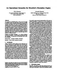
5 Theory of objects and classes Python is an object-oriented language. Values, including built-in values such as integers, strings, and functions, are represented by objects. Objects are mappings of names to addresses. The addresses point to the object’s data and the associated operations (functions). Every object has exactly one class. Even classes, being objects themselves have a class. The class-of relations between object and their classes can be represented by a tree. At the root of such a tree is the class type, which is its own class. See for example Figure ??. Every class has one or more base classes, with the exception of the object object, which has no bases itself. The bases of a class are sorted by their local precedence order. The bases of a class A, the bases of the bases, and so on, are the superclasses of A. The object object is a superclass of all classes. The base-of relation between types can be represented by a directed (from class to base), acyclic graph with edges ordered by their local precedence order. In this inheritance graph, all paths eventually lead to the base object object. See for example Figure ??. Both the class and bases are object attributes: the class of an object is stored in the attribute class , and the bases attribute contains a tuple of a class’ base classes. The order of bases in the bases tuple define the local precedence order. Classes are differentiated from other objects, only by their bases attribute, which ‘normal’ objects lack. All values Θ(a) on a heap Θ have an object representation ΩΘ a . The object representation is the mapping of names to values, i.e. the object’s attributes. The value of an object is determined by the class of an object. For example, objects of class type or object have a value None, and objects of class int have a primitive integer value. The object representations of built-in types and functions, are not stored on the heap. Built-ins have an immutable object representation [ class → aC ], where C is the class of the built-in type. Only a module value returns an object representation extended with its own mapping.

5.1 The method resolution order A class inherits the attributes of its superclasses. Objects have access to the attributes of their class, including the inherited attributes, as if they are their own attributes. However, when classes have different definitions for the same attributes, it is unclear which takes precedence. To resolve conflicts between inherited attributes, we define a so called method resolution order (mro). The order of classes in the mro determines which attribute overrides the other attributes of the same name. Despite the name, the mro determines not only the resolution of methods (function attributes), but the resolution of all attributes.

17

5 Theory of objects and classes

type

object

A

B

b

c

C

Figure 5.1: Example tree showing class-of relations. The classes object, A, B , and C have class type, which is its own class. The objects a and b have classes A and B respectively.

type

object

A

B 2 1 C

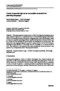
Figure 5.2: Example inheritance graph. The classes type, A, and B inherit from object. The class C inherits A and B , in that order.

18

5.1 The method resolution order object

A

new

B

C

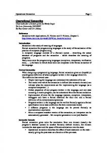
Figure 5.3: A (partial) extended inheritance graph. The marked arrow is added to the inheritance graph in Figure ??. Thus the class C has the mro C , A, B , object. The C3 algoritm Python uses the C3 algorithm originally developed for Dylan [?, ?] to find an mro that satisfies a number of requirements. Most importantly, • The mro observes local precedence order. For example, a class A that precedes a class B in the local precedence order of a class C , must precede B in the mro of C . • The mro is monotonic. For example, a class A in the mro of a class B , must precede B in any mro that contains A. To compute the C3 linearization, the inheritance graph is extended with edges for the local precedence order of bases: for each class with ordered list of bases C we insert an edge from C1 to C2 , an edge from C2 to C3 , and so forth. The ordering of edges is no longer relevant in the extended inheritance graph. The C3 algorithm produces a depth first topological sort of the extended inheritance graph, provided that the extended graph is acyclic. See for example Figure ??. mro Θ(a) = a : b t mro Θ(b1 ) t mro Θ(b2 ) t · · · where b = Θ(ΩΘ a ( bases ))

(5.1)

The mro is defined using a left associative merge operator a t b that merges the two topological sorts a and b. Note that, if a contains a class that is also in b, that class will occur only once in a t b. [] a (a : a) (a : a) (a : a)

t t t t t

b =b [] =a (b : b) if a ≡ b =a :a t b (b : b) if a 6≡ b ∧ a ∈ / b =a :a t (b : b) (b : b) if a ≡ 6 b∧b∈ / a = b : (a : a) t b

(5.2)

Illegal inheritance graphs Not all inheritance graphs are considered legal, e.g., cyclic extended inheritance graphs are not allowed. This sometimes has unintuitive consequences, see for example Figure ??.

19

5 Theory of objects and classes

object

object

1 A

2 2

B

A

1

B

Figure 5.4: The inheritance graph on the right has an illegal ordering of its base classes: the extended inheritance graph has a cycle object → B → object. The inheritance graph on the right is legal, because A inherits B before object and thus has no cycle in its extended inheritance graph. Furthermore, all classes must have at least one base, with the exception of object, and classes cannot have duplicate bases. Only classes can serve as bases. Finally, a class can only have one built-in superclass (e.g. int or list).

5.2 Mappings of inherited attributes As mentioned before, the mro determines what attributes a class inherits. In order to lookup the attributes of an object ΩΘ a , we define two derived mappings that encapsulate the inheritance of attributes. A mapping of class attributes We define the derived mapping of class attributes ΦΘ a to contain the inherited attributes of the class of a and its own attributes. It is defined using a capital version of the join operator ⊕. L Θ The capital join operator Θ a merges the objects ΩΘ a1 through Ωan , where n = |a|. L = ∅L LΘ [ ] a : a = Θ a ⊕ ΩΘ a Θ The derived mapping ΦΘ a is defined as the joined mappings of the mro of the class of a. L ΦΘ a = Θ mro Θ(ac ) where ac = ΩΘ a ( class )

(5.3)

A mapping of all attributes Θ Finally, the full collection of attributes ΥΘ a of an object Ωa is defined as the combination of its inherited attributes and the object’s own attributes.

Θ Θ ΥΘ a = Φa ⊕ Ωa

20

(5.4)

5.3 Classes as types

5.3 Classes as types In the object-oriented world the terms “type” and “classes” are often used interchangeably. In Python, the term “type” is somewhat ambiguously defined. We define two typing relations based on the class-of and base-of relations. The subclass relation Classes are said to be subclasses, or subtypes, of their base classes and the base classes thereof. We define the subclass relation aa > fac() TypeError >>> fac(4) 24 >>> exiting minpy Without a standard library and a foreign function interface, the interpreter cannot be used for many serious applications. However, as a platform of experimentation and testing, the interpreter was invaluable. The interpreter includes a tracer that has proven to be very helpful when debugging the rewrite rules. The tracer prints the changes of the abstract machine state. The following interpreter session shows how the tracer is used. The tracer is first enabled by calling enableTrace() of the sys module. After a simple assignment statement the trace

70

15.2 The interpreter shows how the value 1 is stored at address 1006, and the environment with address 22 is updated (in state 5) with a new mapping. The interpreter always prints the result of the last statement if the result is not None. So when we execute the expression statement a, the value is retrieved (states 7 and 8) and printed (states 10 through 15). >>> import sys >>> sys.enableTrace() state_1 = >>> a = 1 state_3 = state_4 = IntValue 1, envs_2, stack_3, 1006> state_5 = ModValue (fromList [("a",1006),("sys",25)]), []:|:29:|:22, stack_2, 0> >>> a state_7 = state_8 = state_10 = state_11 = state_12 = ?([1006])> state_13 = state_14 = StringValue "1", envs_9, stack_12, 1007> 1 state_15 = Traces usually include a lot of addresses that are hard to keep track of. We implemented address expressions that allow us to handle addresses as first class object in the language for debugging. For example, if we had forgotten what the address 1006 pointed to we can retrieve it by entering the expression statement $1006. >>> $1006 1 >>> exiting minpy The interpreter does not only help when debugging but also provides insight in the semantics. Some aspects of the operational semantics ‘emerge’ from a number of rules. Judging where these emergent semantics occur and exploring their consequences, is often difficult. The interpreter allows us to explore these issues using examples. For example, the interaction of the try-finally statement with the return statement (see Section ??) has some unexpected consequences for the semantics. It is quite hard to infer the semantics of this exceptional case from the rules. Running an example in the interpreter however, immediately reveals the emergent semantics. Our interpreter runs considerably slower than CPython. This is no surprise. We paid little attention to the performance of the interpreter. It should be noted though, that the difference is not a simple constant factor. The heap is implemented with a balanced binary tree, whereas CPython uses a direct mapping of memory

71

15 Conclusion addresses to values. For a simple address lookup, the former has a complexity of O(log(n)), whereas the latter has a constant complexity. Due to the absence of any garbage collector in the interpreter our interpreter uses much more memory than CPython. Indeed, it will be hard to test any memory intensive programs and even a simple program such as while True: pass will eventually crash due to a lack of memory.

15.3 The test suite As mentioned before, our executable operational semantics is testable: we can execute programs and verify whether the minpy interpreter gives the same answer as the CPython interpreter. The CPython implementation is developed with a suite of regression tests. The regression tests could unfortunately not be used to test minpy because it relies on many Python features and libraries that are not available in minpy. Fortunately the efforts to reverse engineer the semantics of CPython provided an excellent opportunity to write new tests. The resulting test suite consists of 134 tests and is completely written in minpy, including the test driver. Beside testing the basic behaviour of constructs, the tests verify aspects such as control flow, order of evaluation, type/class requirements, and variable scoping. Each test covers a single aspect of a single construct. We have been able to run the test suite for a number of implementations of Python (see Table ??). Testing other implementations improves confidence in the tested implementations. Judging from the low number of failed tests across implementations, the other implementations seem to implement the same language, and conversely, minpy and the test-suite seem to capture a common subset of Python. Hopefully minpy can converge on the essential core of Python. Implementations CPython 2.5.2 (reference) minpy PyPy 1.0.0 build 41081 Iron Python 1.1.1 on .net 2.0.50727.42 Jython 2.2.1 on java1.6.0 0

Failed 1 13 3 15 17

Table 15.1: Number of failed tests for various Python implementations. Since CPython is the reference implementation one would expect no errors. There is, however, one test that crashes the Python interpreter completely. The developers of CPython acknowledged that this was a bug and immediately solved the problem. None of the other implementations crashed in the same situation. Our interpreter fails 13 tests, all of which are by definition errors in our semantics. Most of the errors are considered missing features. For example, lists in minpy raise an exception when a negative index is used. CPython on the other hand, treats negative indices as normal indices on the reversed list with an offset of 1. Thus in CPython [1, 2][−1] evaluates to the value 2 but raises an exception in minpy.

72

15.4 Future work Of course there are many more errors in minpy than have been tested or even discovered. Some of the known issues are listed in Section ??. Interpreting the test results of other Python implementations is difficult. Some differences are intentional and can therefore not be considered bugs. Whether or not a failed test indicates a bug is a matter of opinion. Nevertheless we tried to interpret the results somewhat: The PyPy interpreter failed three tests due to incompatibilities only; none of the failures indicated bugs. Iron Python failed quite a number of tests, but only five of those can be considered bugs. Of the failed tests on Jython, only three can be considered bugs.

15.4 Future work There is an enormous body of work that can be based on this operational semantics. First of all, minpy can be expanded to cover all, or at least a more complete subset of Python. The grammar of minpy and therefore the specification, is much simpler than Python’s syntax (see Chapter ??). Most significantly, list and generator comprehensions, keyword arguments and other advanced function parameters, the with statement, and the global statement are missing. Many optional elements and other syntactic sugar are also missing in minpy. This makes the semantics less verbose and allows us to concentrate on the most interesting aspects of Python. Nevertheless, for the sake of completeness, they should eventually be specified. It should be noted that many constructs that could be considered syntactic sugar, actually have semantics that cannot completely be described by a simple transformation. For example, the augmented assignment x + = 1 is not equivalent to x = x + 1: in the former case Python would call the class function iadd , but for the latter it would call setattr and add . We are confident that all constructs of Python that are missing from minpy can be added without significant changes to the existing semantic rules. The structure of the abstract machine will not have to be changed, and the framework used to describe the rules will not need significant extensions. Secondly, there are some errors in the current semantics that should be corrected. The test-suite pointed out some errors in the semantics of class initialization. Although we do use the class of a class –the metaclass– to construct classes, the mechanics of metaclasses have not been covered completely (see Section ??, specifically Rule ??). Most of the built-in types have been specified to make the interpreter usable (see Chapter ??). But the current semantics of minpy’s built-in types are not conform to Python. For example, minpy does not support coercion, and the dictionary class only accepts strings as keys. Thirdly, the scope of the semantics (see Section ??) can be expanded to encompass more of Python’s aspects: • Garbage collection and its interaction with the operational semantics can be explored an formalised. • Concurrent programming, notorious for its complexity, can be formalised. • The interaction of Python with the outside world –the foreign function interface (FFI)– can be specified.

73

15 Conclusion • The various reflective features can be formalised. It seems that most of these features can be specified fairly easily. For example, the dict attribute that exposes the attribute mappings of an object, would not require big changes. For completeness one might consider to add so called old-style classes as well. It might be more productive to update the entire specification to a newer version of Python, that will does not support old style classes. Fourthly, the interpreter, which will benefit from all improvements of the semantics, can be improved. Currently the error feedback is minimal. It would be very useful if raised exceptions also print a stack trace. The performance of the interpreter can probably be improved, but it is doubtful it will ever achieve performance comparable to CPython without compromising the legibility of the semantics. The interpreter could also be used as a basis for various other tools. The current basic tracing functionality could be extended to a fully fledged debugger for example. Finally, our work opens many new avenues of research. The lack of a formal semantics for Python prevented any formal work on Python. Now however we can pursue various new directions of research: • One can prove properties of Python with respect to our semantics. For example, we would very much like to prove that the execution of any possible Python program will never end in a state, other than the final state, that cannot be rewritten. Such a proof would have prevented the bug that we found in CPython. • New tools for and analyses of Python programs can be developed more easily. For example, a tool that type-checks a Python program could be developed. Perhaps some properties of the type system could even be proven correct. • Language extensions can be developed within our framework. Resulting in both a formal description of the extension and a proof of concept interpreter.

74

A Builtin values A.1 The base objects object and type oobject = · [ getattribute , setattr , delattr , new , init , str , bases , class ]

→ object. → object. → object. → object. → object. → object. → a() → atype

otype = · [ getattribute , bases , class , new , call , str ]

→ type. getattribute → a(object,) → atype → type. new → type. call → type. str

getattribute setattr delattr new init str

The default string representation 

, Γ, S, object. str ([aself ])

Θ ⇒ Θ ⊕ [a → ("")], Γ, S, a where a = new address ∈ /Θ (A.1)

Default string representation for classes

 Θ , Γ, S, type. str ([a ]) self

 ⇒ Θ ⊕ [a → ("")], Γ, S, a (A.2) where a = new address ∈ /Θ

75

A Builtin values

A.2 The function and generator ogenerator = · [ class → atype , bases → a(object,) → generator. next , next , send → generator. send , iter → generator. iter ] ofunction = · [ class → atype , bases → a(object,) , call → function. call ]

A function as a callable object



Θ, Γ, S, function. call ([a ]) ⇒ Θ, Γ, S, a

(A.3)

The generator as an iterable 

Θ, γ, S, generator. iter ([aself ]) ⇒ Θ, γ, S, aself

(A.4)

A.3 Integer values The integer class oint [ , , , , , , , , ,

76

=· class bases new add sub mul div divmod floordiv pow

→ atype → a(object,) → int. new → int. add : [aint , aint ] → int. sub : [aint , aint ] → int. mul : [aint , aint ] → int. div : [aint , aint ] → int. divmod : [aint , aint ] → int. floordiv : [aint , aint ] → int. pow : [aint , aint ]

A.3 Integer values , , , , , , , ]

neq eq lt le gt ge str

→ int. → int. → int. → int. → int. → int. → int.

neq eq lt le gt ge str

: [aint , aint ] : [aint , aint ] : [aint , aint ] : [aint , aint ] : [aint , aint ] : [aint , aint ] : [aint ]

Literal integers Evaluating an integer literal

 Θ , Γ, S, i

 ⇒ Θ ⊕ [a → i ], Γ, S, a where a = new address ∈ /Θ

(A.5)

Integer primitives The addition primitive



Θ, Γ, S, int. add ([ax , ay ]) ⇒ Θ, Γ, S, (Θ(ax ) + Θ(ay ))

(A.6)

The equals primitive



Θ, Γ, S, int. eq ([ax , ay ]) ⇒ Θ, Γ, S, Θ(ax ) ≡ Θ(ay )

(A.7)

The constructor primitive

 , Γ, S, int. new ([ac ])

Θ ⇒ Θ ⊕ [a → o ], Γ, S, a where a = new address ∈ /Θ o = ([ class → ac ], 0)

The string representation

 Θ , Γ, S, int. str ([a ]) o

 ⇒ Θ ⊕ [a → (show Θ(ao ))], Γ, S, a where a = new address ∈ /Θ

(A.8)

(A.9)

77

A Builtin values

A.4 Booleans The boolean class bool = · [ class , bases , nonzero , str ]

→ atype → a(object,) → bool. nonzero : [abool ] → bool. str : [abool ]

Literal booleans Evaluating a boolean literal

 Θ , γ, S, b

 ⇒ Θ ⊕ [a → (b)], γ, S, a where a = new address ∈ /Θ

(A.10)

Boolean primitives The boolean to boolean conversion primitive



Θ, γ, S, bool. nonzero ([a ]) ⇒ Θ, γ, S, a

The boolean to string conversion primitive

 Θ, γ, S, bool. str ([a ])  

Θ, γ, S, "True"  if Θ(a) ⇒

Θ, γ, S, "False" otherwise

A.5 Strings The string class ostring = · [ class , bases , new , add , mul

78

→ atype → a(object,) → str. new → str. add : [astr , astr ] → str. mul : [astr , aint ]

(A.11)

(A.12)

A.5 Strings , len , eq , getitem , str , "append" ]

→ str. → str. → str. → str. → str.

len : [astr ] eq : [astr , astr ] getitem : [astr , aint ] str : [astr ] add : [astr , astr ]

Literal strings Evaluating a string literal

 , γ, S, t 

Θ ⇒ Θ ⊕ [a → t ], γ, S, a where a = new address ∈ /Θ

(A.13)

String primitives The string constructor primitive

 , γ, S, str. new ([ac ])

Θ ⇒ Θ ⊕ [a → o ], γ, S, a where a = new address ∈ /Θ o = ([ class → ac ], [ ])

The string constructor primitive with starting string 

new ([a , a ]) Θ , γ, S, str. c str

 ⇒ Θ ⊕ [a → o ], γ, S, a where a = new address ∈ /Θ o = ([ class → ac ], Θ(astr ))

The length of string primitive



Θ, γ, S, str. len ([a ]) ⇒ Θ, γ, S, (|Θ(a)|)

The string addition operator primitive

 , γ, S, str. add ([aself , aother ])

Θ ⇒ Θ ⊕ [a → s ], γ, S, a where s = (Θ(aself ) + + Θ(aother )) a = new address ∈ /Θ

(A.14)

(A.15)

(A.16)

(A.17)

79

A Builtin values The string equals primitive 

eq ([a , a ]) Θ, γ, S, str. x y

 ⇒ Θ, γ, S, Θ(ax ) ≡ Θ(ay )

The string get character at index primitive

 Θ , γ, S, str. getitem ([aself , ai ])  

Θ ⊕ [a → [s !! i ]], γ, S, a

 if i < |s| ⇒ Θ , γ, S, raise aIndexError () otherwise where i = Θ(ai ) s = Θ(aself ) a = new address ∈ /Θ

The string to string conversion primitive 

, γ, S, str. str ([ao ])

Θ ⇒ Θ ⊕ [a → Θ(ao )], γ, S, a where a = new address ∈ /Θ

(A.18)

(A.19)

(A.20)

A.6 Lists The list class olist = · [ class , bases , delitem , getitem , setitem , new , add , len , iter , append ]

→ atype → a(object,) → list. delitem : [alist , aint ] → list. getitem : [alist , aint ] → list. setitem : [alist , aint ] → list. new → list. add → list. len → list. iter → list.append

Literal strings Evaluating a list literal

Θ , γ, S , 

Θ , γ, S|[◦, es 0 ], ⇒

Θ ⊕ [a → [ ]], γ, S , where a = new address ∈ /Θ

80

 [e]  e  if e = (e : es 0 ) a otherwise

(A.21)

A.6 Lists

Evaluating the elements of a list literal

 Θ , γ, S|[a, ◦, e] ,a  

0 ], e + + [a ], ◦, es if e = (e : es 0 ) Θ , γ, S|[a  ⇒

Θ ⊕ [a 0 → [a + + [a ]]], γ, S , a 0 otherwise 0 where a = new address ∈ /Θ

(A.22)

List primitives The list constructor primitive 

new ([a ]) Θ , γ, S, list. c

 ⇒ Θ ⊕ [a → o ], γ, S, a where a = new address ∈ /Θ o = ([ class → ac ], [ ])

The length of list primitive 

len ([a ]) Θ, γ, S, list.

 ⇒ Θ, γ, S, (|Θ(a)|)

The get item at index primitive

 Θ, γ, S, list. getitem ([aself , ai ])  

Θ, γ, S, a !! i  if i < |a| ⇒

Θ, γ, S, raise aIndexError () otherwise where i = Θ(ai ) a = Θ(aself )

The set item at index primitive

 Θ , γ, S, list. setitem ([aself , ai , a ])  

Θ ⊕ [aself → a0 ], γ, S, aNone

 if i < |a| ⇒ Θ , γ, S, raise aIndexError () otherwise where i = Θ(ai ) a = Θ(aself ) a0 = [· · · , ai−1 , a, ai+1 , · · ·]

(A.23)

(A.24)

(A.25)

(A.26)

81

A Builtin values The delete item at index primitive

 Θ , γ, S, list. delitem ([aself , ai ])  

Θ ⊕ [aself → a0 ], γ, S, aNone

 if i < |a| ⇒ Θ , γ, S, raise aIndexError () otherwise where i = Θ(ai ) a = Θ(aself ) a0 = [· · · , ai−1 , ai+1 , · · ·]

The append to list primitive

 Θ , γ, S, list.append([a , a ]) self 

⇒ Θ ⊕ [aself → a], γ, S, aNone where a = [Θ(aself ) + + [a ]]

The list addition operator primitive

 , γ, S, list. add ([aself , aother ])

Θ ⇒ Θ ⊕ [a → a], γ, S, a where a = [Θ(aself ) + + Θ(aother )] a = new address ∈ /Θ

(A.27)

(A.28)

(A.29)

A.7 Tuples A.8 The tuple class otuple = · [ class , bases , getitem , new , len ]

→ atype → a(object,) → tuple. getitem : [atuple , aint ] → tuple. new → tuple. len

Literal tuples Evaluating a tuple literal

Θ , γ, S , 

Θ , γ, S|(◦, es 0 ), ⇒

Θ ⊕ [a → (, )], γ, S , where a = new address ∈ /Θ

82

 (e)  e  if e = (e : es 0 ) a otherwise

(A.30)

A.9 Dictionaries Evaluating the elements of a tuple

Θ , γ, 

Θ , γ, ⇒

0 Θ ⊕ [a → (a + + [a ])], γ, where a 0 = new address ∈ /Θ

literal S|(a, ◦, e)

,a



 S|(a ++ [a ], ◦, e0 ), e  if e = (e : e0 ) S , a 0 otherwise

(A.31)

Tuple primitives The tuple constructor primitive 

new ([a ]) Θ , γ, S, tuple. c

 ⇒ Θ ⊕ [a → o ], γ, S, a where a = new address ∈ /Θ o = ([ class → ac ], ([ ]))

The length of tuple primitive

 Θ, γ, S, tuple. len ([a ])

 ⇒ Θ, γ, S, (|Θ(a)|)

The get item at index primitive

 Θ, γ, S, tuple. getitem ([aself , ai ])  

Θ, γ, S, a !! i  if i < |a| ⇒

Θ, γ, S, raise aIndexError otherwise where i = Θ(ai ) a = Θ(aself )

(A.32)

(A.33)

(A.34)

A.9 Dictionaries Dictionary class odict = · [ class , bases , getitem , setitem , delitem , new ]

→ atype → a(object,) → dict. getitem : [adict , astr ] → dict. setitem : [adict , astr , aobject ] → dict. delitem : [adict , astr ] → dict. new

83

A Builtin values

Dictionary literals Evaluating a dictionary literal

 Θ , γ, S ,e  

e , tail e}, e Θ , γ, S|{∅, ◦ : 1;2 1;1  if |e| > 0 ⇒

Θ ⊕ [a → ∅], γ, S ,a otherwise where a = new address ∈ /Θ

(A.35)

Evaluating the value of a key-value pair

 Θ, γ, S|{d , ◦ : e , e}, a v k

 ⇒ Θ, γ, S|{d , ak : ◦, e}, ev

Evaluating key-value pairs in a

Θ , 

Θ , ⇒

Θ ⊕ [a → d ⊕ [k → av ]], where a = new address ∈ /Θ k = Θ(ak )

(A.36)

dictionary literal γ, S|{d , ak : ◦, e}

, av



 γ, S|{d ⊕ [(k → av )], ◦ : e1;2 , tail e}, e1;1  if |e| > 0 γ, S ,a otherwise (A.37)

Dictionary primitives The dictionary constructor primitive

 Θ , γ, S, dict. new ([a ]) c

 ⇒ Θ ⊕ [a → ([ class → ac ], ∅)], γ, S, a where a = new address ∈ /Θ

The dictionary constructor primitive with starting dictionary

 , γ, S, dict. new ([ac , ad ])

Θ ⇒ Θ ⊕ [a → ([ class → ac ], Θ(ad ))], γ, S, a where a = new address ∈ /Θ

The set item with key primitive

 , γ, S, dict. setitem ([aself , ai , av ])

Θ ⇒ Θ ⊕ [aself → d 0 ], γ, S, aNone where k = Θ(ai ) d 0 = (ΩΘ aself , Θ(aself ) ⊕ [k → av ])

84

(A.38)

(A.39)

(A.40)

A.9 Dictionaries The get item with key primitive 

Θ, γ, S, dict. getitem ([aself , ai ])  

Θ, γ, S, Θ(aself )(i ) if i ∈ Θ(aself )

 ⇒ Θ, γ, S, raise aIndexError otherwise where i = Θ(ai )

The delete item with key primitive 

, γ, S, dict. delitem ([aself , ai ])

Θ ⇒ Θ ⊕ [aself → d 0 ], γ, S, aNone where k = Θ(ai ) d 0 = (ΩΘ aself , Θ(aself ) k )

(A.41)

(A.42)

85

A Builtin values

86

Rules

87