Department of Computer Science, Rice University, Houston Texas ... of list scheduling in light of available parallelism, the list scheduling priority heuristic, and ...
An Experimental Evaluation of List Scheduling Keith D. Cooper, Philip J. Schielke, and Devika Subramanian Department of Computer Science Rice University Houston, Texas, USA
Rice Computer Science Techcnical Report 98-326 September 1998
An Experimental Evaluation of List Scheduling
⋆
Keith D. Cooper, Philip J. Schielke, and Devika Subramanian Department of Computer Science, Rice University, Houston Texas
Abstract. While altering the scope of instruction scheduling has a rich heritage in compiler literature, instruction scheduling algorithms have received little coverage in recent times. The widely held belief is that greedy heuristic techniques such as list scheduling are “good” enough for most practical purposes. The evidence supporting this belief is largely anecdotal with a few exceptions. In this paper we examine some hard evidence in support of list scheduling. To this end we present two alternative algorithms to list scheduling that use randomization: randomized backward forward list scheduling, and iterative repair. Using these alternative algorithms we are better able to examine the conditions under which list scheduling performs well and poorly. Specifically, we explore the efficacy of list scheduling in light of available parallelism, the list scheduling priority heuristic, and number of functional units. While the generic list scheduling algorithm does indeed perform quite well overall, there are important situations which may warrant the use of alternate algorithms.
1
Introduction
Instruction scheduling plays a critical role in determining the performance of compiled code on today’s computers. Today’s microprocessors rely on the compiler to hide memory latencies and to keep functional units busy—both are tasks for the instruction scheduler. On the microprocessors of tomorrow, the quality of instruction scheduling may be more important, since these machines will feature longer memory latencies and more functional units. Despite the importance of scheduling, we know quite little about the behavior of list scheduling—the most widely used technique for instruction scheduling [1, 3]. This paper presents an experimental evaluation of list scheduling that attempts to answer the following questions: 1. Is there room for improvement beyond list scheduling? It is widely believed that list scheduling usually achieves optimal or near-optimal results [5]; is this the case? 2. Will new microprocessor designs change the efficacy of list scheduling? To keep these machines busy, compilers will apply transformations that increase instruction-level parallelism; how will that change the scheduling problems that the compiler sees? 3. Can we classify scheduling problems so that the compiler can recognize when other scheduling techniques should be invoked? If we can discover metrics that predict bad behavior from list scheduling, we can design compilers that avoid it. To answer these and other questions, this paper examines the strengths and weaknesses of list scheduling. We develop several metrics to classify instances of scheduling problems. We evaluate the performance of list scheduling against those metrics and compare it against two alternative scheduling algorithms. Our experiments use both real benchmark codes and randomly-generated sets of basic blocks. The remainder of the paper is organized as follows. Section 2 provides background information about the framework in which we performed this investigation. Section 3 discusses the list scheduling algorithm. Section 4 describes improvements to list scheduling and an alternative technique based on iterative repair. Section 5 presents our metrics for classifying instances of the scheduling problem. Sections 6 and 7 present experimental results.
2
Experimental Setup
Our experiments use components of a research compiler system developed at Rice University. It has front ends for both C and Fortran; these translate the input code into a linear, low-level intermediate form called iloc. ⋆
This work has been supported by DARPA and the USAF Research Laboratory through Award F30602-97-2-298.
The individual iloc operations resemble simple risc machine operations, with register-to-register operations that manipulate virtual registers, plus load and store operations. Individual operations are grouped together into instructions; an instruction aggregates together all the operations that begin execution in a single cycle. Before scheduling, the compiler applies a series of optimizations to the iloc code. This includes pointer analysis, dead code elimination, global value numbering, lazy code motion, constant propagation, strength reduction, register coalescing, dead code elimination, and empty block removal. For the purposes of this paper, no register allocation was performed; this eliminates interactions between allocation and scheduling and isolates the impact of scheduling. After optimization, the compiler passes the code to the scheduler. Each block is scheduled individually. The first step constructs a data-precedence graph (dpg) for the block. The dpg G = (N, E, E ′ ) has a node n ∈ N for each operation. Edges e = (ni , nj ) ∈ E represent dependences between operations; their direction matches the flow of values. Edges in E ′ represent anti-dependences in the code that prevent reordering. An anti-edge e = (ni , nj ) ∈ E ′ indicates that moving nj before ni would change the flow of values because of a name that ni uses and nj redefines. The details of the individual schedulers vary; they are described in sections 3 and 4. To evaluate the schedules, we use several variations on a simple processor model. Each architecture consists of k identical pipelined functional units. Each functional unit can execute any iloc operation. For our experiments, we vary k between one and three. Each iloc operation has a latency—the number of cycles required before its results are available. Register values are read in the cycle when the instruction begins execution, and results are defined in the last cycle of its latency. Thus, an operation u can begin execution when all operations v |(v, u) ∈ E have completed, and all operations w |(u, w) ∈ E ′ have already been issued.
3
The List Scheduling Algorithm
Here we describe our implementation of list scheduling. First, the dpg is built as described in the previous section. Next, priorities are assigned to each node in the graph. There are several different heuristics that can be used to assign priorities. A common and effective strategy is to use the latency weighted depth of the node [3, 5]. The depth of a node n is the length (number of nodes) of the longest path in the dpg from n to some leaf (including n and the leaf.) The latency weighted depth is computed the same way, but the nodes along the path are weighted using the latency of the operation the node represents. The following formula summarizes the priority computation for a node n:
priority(n) = max ∀l∈leaves(DP G) ∀p∈paths(n,...,l)
l X
pi =n
!
latency(pi )
Dynamic programming can be used to compute the priorities efficiently, and we take into consideration the anti-edges described above: if n is a leaf. latency(n) priority(n) = max(latency(n) + max(m,n)∈E (priority(m)), max(m,n)∈E ′ (priority(m))) otherwise.
The final phase is the actual list scheduling algorithm that constructs the schedule for the block. Starting at cycle 0, the list scheduler places operations into the schedule cycle by cycle. Any operation that is “ready” at cycle X (i.e. all its operands have been computed), is a candidate to be scheduled at cycle X. The priorities computed in the previous step are used to determine which ready operation to schedule, by selecting the highest priority operation first. Any tie in the priority of two operations is broken arbitrarily. The algorithm is detailed in Figure 1. Through the rest of the paper we refer to this algorithm as ls.
4
List Scheduling Alternatives
Here we present two alternatives to the ls algorithm discussed in the last section. For a survey of scheduling techniques see [4, 8]. A machine learning approach to scheduling has been developed by Moss and others [7].
Input: Data Precedence Graph (N,E,E’) with priorities assigned to each node. Parameters of machine (instruction latencies, pipelining, number of functional units, etc.) Output: A schedule containing all nodes in the graph that satisfies the precedence constraints in the DPG and the resource constraints of the machine. Algorithm: cycle = 0 ready-list = root nodes in DPG inflight-list = empty list while ( ready-list or inflight-list not empty, and an issue slot is available ) for op = (all nodes in ready-list in descending priority order) if (a functional unit exists for op to start at cycle) remove op from ready-list and add to inflight-list add op to schedule at time cycle if (op has an outgoing anti-edge) Add all targets of op’s anti-edges that are ready to ready-list endif endif endfor cycle = cycle + 1 for op = (all nodes in inflight-list) if (op finishes at time cycle) remove op from inflight-list check nodes waiting for op in DPG and add to ready-list if all operands available endif endfor endwhile Fig. 1. List Scheduling algorithm
4.1
Random Tie Breaking
A traditional list scheduler returns a single solution by breaking any ties in the priority of two or more operations arbitrarily. By running the list scheduler several times and breaking ties randomly, we could potentially generate more and better solutions. Figure 2 is an example from the tomcatv benchmark. Assume all load immediates (LDI) take one cycle, all add operations (ADD) take two cycles, and the copy (i2i) takes one cycle. Assume we are scheduling on a machine with two identical functional units. The numbers next to the operations are the priority values that list scheduling uses. In this figure we see two different list schedules that could be generated from the dpg. The second one requires one less cycle. The critical decision comes in the second cycle, where the tie between the LDId and LDIc must be broken. Scheduling LDId early enough results in a shorter schedule. 4.2
Backward list scheduling
In addition, there are some blocks for which a backward list scheduler can generate a better solution. A backward list scheduler works by reversing the direction of all edges in dpg, and scheduling the finish times of each operation. (Note that the start time of operations must be used to ensure enough available functional units for a given cycle.) This technique tends to cluster operations toward the end of the schedule instead of the beginning like a forward list scheduler. For an example of a block that benefits from backward list scheduling see Figure 3, which shows a block from the go benchmark. Assume there are two integer units that can execute the LDI operations (one cycle), the LSL operation (one cycle), the ADD operations (two cycles), ADDI operation (one cycle), and the CMP operation (one cycle). A separate memory unit executes the ST operations (four cycles). All functional units are completely pipelined. A forward list scheduler will schedule the four LDI operations and the the LSL before scheduling any of the ADD operations. This delays the start of the higher latency store operations (ST). A better schedule can be found by a backward list scheduler as shown in the example.
6
LDIa 4
5
4
4
LDIb ADDa LDIc 2
i2i
LDId
3
3
ADDb
ADDc LDIe ADDd
2
3
1JMP
Two possible list schedules LDIa LDIb ADDa LDIc LDId i2i ADDb ADDc ADDd LDIe --JMP
LDIa ADDa LDIc ADDb i2i JMP
LDIb LDId ADDd ADDc LDIe
Fig. 2. Example block from tomcatv
8
8
8
LDIa LSL 7
8
8
LDIb LDIc LDId
7
7
7
7
ADDa ADDb ADDc ADDd ADDI 2
5
CMP
STa
5
5
STb
5
STc
5
STd
STe
1 BR
Forward List LDIa LDIb LDId ADDb ADDd CMP
LSL LDIc ADDa ADDc ADDI
-------
Backward List
STa STb STc STd STe
LDId ADDI ADDd ADDc ADDb ADDa
LSL LDIc LDIb LDIa
STe STd STc STb STa
----CMP BR
BR Fig. 3. Example block from go, showing the benefits of backward list scheduling.
Input: Data Precedence Graph. Parameters of machine (instruction latencies, pipelining, number of functional units, etc.). The number of iterations to perform iter. Output: A schedule containing all nodes in the graph that satisfies the precedence constraints in the DPG and the resource constraints of the machine. Algorithm: min = largest integer shortest is a schedule initially empty for x = (1 to iter) Create an initial schedule by scheduling all operations as early as possible subject to precedence constraints. while (there exist resource conflicts in schedule) conflict time = the cycle of the first resource conflict in the schedule (1) select an operation that has a resource conflict at conflict time unschedule operation and all its successors in dpg (2) reschedule operation and its successors later in schedule. endwhile if length of schedule is less than min then min = length of schedule shortest = schedule endif endfor Fig. 4. Basic Iterative Repair Scheduling algorithm
We have developed a new scheduling technique called rbf (randomized backward and forward list scheduling.) rbf schedules each block M times forward and M times backward breaking any ties in the priority heuristic randomly. The shortest schedule over all 2M runs is kept. The best value for M should be determined based on the characteristics (e.g. number of operations) of the particular scheduling problem. 4.3
Iterative Repair Scheduling
Here we introduce the application of a repair based scheduling technique called “iterative repair” to the problem of instruction scheduling in a compiler. This algorithm comes from the AI community and is described by Lin and Kernighan [6], and Zweben, et. al. [10, 11]. The technique has shown promise for several scheduling problems including space shuttle mission scheduling. The generalized algorithm is presented in figure 4. The idea is straightforward. First, create an instruction schedule that begins each operation as early as possible with respect to the precedence constraints of the dpg, but ignores the resource constraints imposed by the limited number of processing elements. Now “repair” the schedule by moving operations that have a resource conflict to a point later in the schedule. This reduces the number of resource conflicts for the cycle being repaired. A resource conflict is simply a point in the schedule where more operations are scheduled than the available number of functional units. The earliest cycle with a conflict is found, and one of the conflicting operations is selected (line (1) in the algorithm). This operation and all operations that depend on it are removed from the schedule (called unscheduling). The selected operation and its dependent operations are then inserted back into the schedule (called rescheduling) at a later point (line (2) in the algorithm). We continue repairing the schedule until there are no more resource conflicts. The algorithm is run a “user specified” number of times, and the shortest schedule over all the trials is selected as the final schedule. We have tested several new variations of the iterative repair scheduling algorithm. The most effective one to date we refer to as ir-bias. In ir-bias the selection of which node to move (called the move-node) is not completely random. Rather, operations with lower priority values (the same priority values as used by the list scheduler) are more likely to be moved. The selection is probabilistic; the probability that a node is selected is inversely related to its priority. The move-node is scheduled one cycle later than its original position. All successor nodes are rescheduled as early-as-possible with respect to this new start time. This could cause additional conflicts to be created
later in the schedule, but a future repair will correct any new conflicts. After each repair we compare the length of the new schedule to that of the old schedule. If the new length is greater, the repair is ignored, the state of the previous schedule is restored, and a new move-node is selected. A new schedule with a greater length than the previous schedule is kept ten per cent of the time to avoid local minima. For more information on iterative repair algorithms please see our technical report [9].
5
Metrics Used in Experiments
In this section we define several metrics that help us to characterize scheduling problems. The first is used to help us assess the quality of a schedule generated for a particular graph. The second and third metrics are used to assess the difficulty of a particular scheduling problem instance. 5.1
Minimum Schedule Length
We would like to be able to evaluate the performance of our scheduling algorithms on particular problem instances. One way to do this is to estimate the minimum possible schedule length for the problem. Of course finding the minimum length is NP-complete but we use several observations to develop a lower bound on the minimum schedule length. If our scheduler returns a schedule whose length is equal to this metric we are guaranteed that the solution is optimal. The first part of our estimate is the critical path length of the dpg denoted by cpl(G) where G is the dpg. This is the length (in cycles) of the longest (latency weighted) path from any leaf in the dpg to any root. Since any schedule must ensure all dependences in the dpg are followed, there exists no valid schedule whose length is less than the critical path length. Thus, if a scheduling algorithm finds a schedule whose length equals the critical path length for a particular problem, no more work on that problem will result in a better schedule. Since critical path length does not take hardware constraints into account, we refine this minimum schedule length estimate in the following way. Assume we schedule every operation in the dpg as early as possible without regard to hardware constraints (i.e. the starting point for iterative repair.) The length of this schedule is equal to the critical path length cpl(G) . Next we find all nodes on some critical path. These nodes are important because if any one of them gets scheduled later than its as-early-as-possible position, the final schedule length will be greater than the critical path length. Finally, we examine the schedule cycle by cycle and record the maximum number of critical operations scheduled to start at any one cycle (call this value N ′ .) Let p be the number of processing elements on the machine. If N ′ is greater than p, then the minimum schedule length must be at least cpl(G) + ⌈N ′ /p⌉ − 1. One final measure we use for the minimum schedule length is simply the number of operations N in the dpg divided by the number of available processing elements p. The following equation summarizes our estimate for minimum schedule length of a dpg G. minlength(G) = max(cpl(G) + ⌈N ′ /p⌉ − 1, N/p) 5.2
Available Parallelism
This metric is a measure of how much parallelism is available in a piece of code. It is similar to the available speedup measure described by Rau and Fisher [8], except that we compute the value during compilation. Different dpg’s have differing amounts of parallelism available in them. To quantify this notion we define a metric called the available parallelism or ap of a dpg. This value is equal to the length of the worst possible schedule (i.e. the sum of the latencies of all operations in the dpg) divided by the length of the best possible schedule (i.e. the critical path length). Of course this value is dependent on the latencies of the various operations as determined by the architecture. There is an interesting correlation between available parallelism and the difficulty of a particular scheduling problem. This relationship is explored in section 7. Intuitively, the lower the ap the fewer decisions any scheduling algorithm needs to make, while higher ap values lead to more decisions. 5.3
Number of List Schedules
This metric is another attempt to quantify the number of decisions made by ls. In this metric we estimate the number of possible list schedules caused by ties in the priority heuristic. Consider an architecture with
two identical functional units. Assume the list scheduler is at a point where four operations are tied for the highest priority value and are data ready. There are 4 choose 2 or 6 possible schedules that could result from this tie. If there are no ties to be broken by either forward or backward list schedulers, then rbf will yield no improvement. The metric num list estimate is an estimate of the number of possible list schedules and is computed while running ls. It’s initial value is one, and it is updated every time a tie is encountered while scheduling. Let max be the number of nodes in the ready list with highest priority, and p be the number of processing elements still available this cycle. To update num list estimate we do the following: � � max num list estimate = num list estimate ∗ p
6
Experimental Results on Real Code
In this section we discuss the effectiveness of the various schedulers on benchmark codes. A summary of the benchmark codes is presented in table 1. In the table we show the number of iloc operations, average number of operations per basic block, the average available parallelism per block, and the maximum available parallelism over all blocks. All available parallelism numbers are rounded to the nearest tenth. Notice that most of the blocks are small. Over all benchmarks, about 56 per cent (11412 of 20561) of basic blocks had available parallelism values equal to 1. About 0.6 per cent (131 of 20561) had available parallelism values greater than 5.0. The distribution of available parallelism for the remainder of the blocks is shown in figure 5. Notice that on the average there is little available parallelism, although a few blocks do have very high available parallelism values. Table 1. Benchmark Statistics Benchmark operations ops per block avg. ap max ap adpcm 339 4.1 1.3 6.0 clean 7902 5.5 1.3 5.5 compress 1281 5.6 1.4 8.6 fft 1544 6.4 1.5 6.5 go 50401 5.0 1.2 12.5 gzip 10264 4.9 1.4 7.5 jpeg 13029 6.6 1.3 11.4 shorten 5746 4.2 1.2 9.5 water 3509 11.6 1.7 23.6 applu 9798 16.6 1.9 25.1 cg 589 6.6 1.4 3.5 doduc 19439 12.4 1.9 74.9 fpppp 8627 27.5 2.2 46.6 mg 1789 11.1 1.8 10.9 tomcatv 684 13.4 2.3 10.0
Table 2 shows a lower bound on the percentage of basic blocks that ls was able to schedule optimally on the various architectures. That is, the percentage of basic blocks for which ls found a schedule whose length equaled minlength(G), where G is the dpg constructed for the basic block. These numbers are quite high and indicate that ls is very often finding the optimal schedule. Each benchmark was scheduled using rbf and ir-bias, on architectural models with one, two, and three identical processing elements. rbf was run 50 times backward and forward, and ir-bias was run 100 times. The runtime performance of the resulting code was compared to that of the code scheduled with ls. Very few improvements were observed. tomcatv improved by .6 per cent on one processing element and .4 per cent on three processing elements. doduc improved by .1 per cent on one processing element. All other codes were sped up by less than .1 per cent when the more powerful scheduling algorithms were used. In roughly 55 per cent of the experiments no speed up was observed. Clearly ls performs quite well on real codes when scheduling is performed at the basic block level. Few improvements were observed when using more powerful scheduling techniques. The next section presents further evidence as to why that is the case.
Available Parallelism for Benchmark Codes 1600
1200 1000 800 600 400 200
6
9
2
5
8
1
4
7
2.
3.
3.
3.
4.
4.
4.
5
3
2.
7 1.
2
4
2.
1
1.
0
1.
Number of Blocks
1400
Parallelism
Fig. 5. Available Parallelism vs. Number of Blocks
Table 2. Percentage of Basic Blocks Optimally Scheduled by ls
Benchmark adpcm clean compress fft go gzip jpeg shorten water applu cg doduc fpppp mg tomcatv
Proc. one 97.6 91.4 89.0 91.7 93.9 91.3 94.2 96.3 85.8 86.8 91.0 82.1 85.0 91.3 88.2
Elements two three 96.3 98.8 97.7 99.2 93.4 97.8 95.0 98.3 97.5 99.3 95.7 98.9 97.1 99.1 96.4 99.3 94.1 96.7 87.1 92.5 95.5 97.8 92.2 97.9 92.7 96.8 93.8 97.5 70.6 80.4
10 ops, 1 proc
10 ops, 1 proc, IR wins
12
1.6 1.4
% of IR wins
8 6 4 2
1.2 1 0.8 0.6 0.4 0.2
2
4
8
4.
6
3.
4
4
3.
4.
2
3.
8
3.
6
Parallelism
3
4
8 1.
2.
6 1.
2
4 1.
2.
2 1.
2.
4
2
2
8
4.
6
4.
4
3.
4
2
3.
8
3.
6
3.
4
2.
3
2
2.
8 1.
2.
6 1.
2.
4 1.
2
2
0
1.
0
2.
% non-optimal
10
Parallelism
20 ops, 1 proc
20 ops, 1 proc, IR wins
16
2.5 2
12
% of IR wins
% non-optimal
14
10 8 6 4
1.5 1 0.5
2
3
6
9
4.
4.
8 2.
4.
5 2.
4
2 2.
7
9 1.
4
6 1.
3.
3 1.
5
8
1
4
4.
5.
5.
7 2.
2
4 2.
4.
1 2.
9
8 1.
4.
4 5.
6
1 5.
3.
8 4.
3
5 4.
3.
2 4.
3.
9 3.
Parallelism
3
6 3.
% of IR wins 3
7 2.
4.5 4 3.5 3 2.5 2 1.5 1 0.5 0
3.
4 2.
3
1 2.
% non-optimal
50 ops, 1 proc, IR wins
20 18 16 14 12 10 8 6 4 2 0
8
3.
9 4.
Parallelism
50 ops, 1 proc
1.
1
6 4.
Parallelism
3.
3 4.
4
7
8 2.
4
5 2.
3.
2 2.
3.
9 1.
1
6 1.
3.
3
0
1.
0
Parallelism
Fig. 6. Results for 1 processing element
7
Experimental Results on Random Graphs
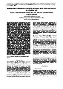
In this section we present some experimental results for instruction scheduling on randomly generated basic blocks with different numbers of operations. Each iloc operation was randomly assigned a latency between 1 and 4 cycles with uniform distribution. Each operation had two source registers and a single destination register. Each register number was chosen randomly. Each graph was first scheduled using ls. The resulting schedule length was compared against the minlength metric described in section 5. If the schedule length was greater than minlength the graph was scheduled with rbf run 50 times backward and forward and ir-bias run 1000 times. The results for scheduling on one processing element are shown in figure 6. The left-hand graphs plot available parallelism on the x-axis and the percentage of experiments where either rbf or ir-bias found a shorter schedule than ls on the y-axis. Blocks with 10, 20 and 50 operations are shown. This value is a lower bound on the percentage of times ls failed to find the optimal schedule. A minimum of 2000 graphs were scheduled at each parallelism level. The right-hand graph shows the percentage of experiments in which ir-bias found a shorter schedule than both rbf and ls. Note the interesting shape of the graphs. Clearly list scheduling performs better at certain levels of available parallelism than others. It is easy to explain list scheduling’s success at low levels of available parallelism. When the list scheduler has very few choices to make, its probability of making an incorrect tie-breaking decision is low. One might then expect that with the exponential increase in the number of scheduling decisions at higher levels of available parallelism, list scheduling would have a greater probability of making incorrect decisions. Interestingly that is not the case; list scheduling performs well at high levels of available parallelism.
20 ops, 1 proc Unique schedule lengths
1.6 1.5 1.4 1.3 1.2 1.1
1
4
7
4.
4.
4.
6
8 3.
3
5 3.
5.
2 3.
5.
9 2.
5
6 2.
1
Parallelism
Fig. 7. Number of Unique Schedule Lengths as a Function of Available Parallelism
A possible explanation for the phenomenon is that most of the tie-breaking choices at high levels of available parallelism yield schedules that have the same length. Thus, the choices are really equivalent and do not contribute to list scheduling making incorrect tie-breaking choices. To test this potential explanation we experimentally determined the average number of distinct schedule lengths1 for each value of available parallelism for 20 operations and a single functional unit. The results are in Figure 7. We see that the number of distinct schedule lengths peaks at an available parallelism of about 2.7, corresponding closely to the observed peak in the percentage of times list scheduling is non-optimal. Note further that the number of distinct schedule lengths falls rapidly to 1, indicating that all the different choices of breaking ties yield schedules of the same length. Loosely speaking, we can paraphrase this result as follows — when the available parallelism is high, any decision will do, and thus the probability of list scheduling making an error is again low. Substantial improvements over list scheduling are however possible at a range of parallelism levels with the peak appearing to be around 2.5 to 2.7. Notice further that as the number of operations is increased ls has a more difficult time finding the best solution. Also notice that most of the improvements were found by rbf with M = 50. The picture changes slightly when we increase the number of processing elements as seen in figure 8. As we increase the number of processing elements the graphs “spread out”. For two processing elements the peak appears around 5 to 5.2, about double what it was for one processing element. We are conducting further experiments to explain this near-linear shift in the peaks of the graphs as the number of processing elements increases. Figure 9 plots available parallelism on the x-axis, number of list schedules (see Section 5.3) on the y-axis and the percentage of experiments where rbf or ir-bias beat ls on the z-axis (20 operations, two processing elements). The graph shows that even at low levels of available parallelism if the list scheduler is breaking a lot of ties, it may find a non-optimal schedule.
8
Conclusions
In this paper, we have studied the effectiveness of list scheduling on real codes and on randomly generated graphs. Our observations showed that, in general, list scheduling performs very well on real codes, and there appears to be little opportunity for improving its performance when scheduling over basic blocks taken from these codes. Our experiments on randomly generated blocks provide deeper insight into the conditions where list scheduling is most likely to produce less than optimal schedules. We found that ls has difficulty finding optimal schedules for codes with a moderate amount of available parallelism—the peak difficulty varies with both the number of processing elements and the schedule length. This answers our third question: we have characterized the set of blocks where the compiler writer may want to try other scheduling methods. This suggests a multi-level approach to scheduling, where the compiler uses statistical information about the 1
We used RBF running 5000 time backward and forward to compute the results.
20 ops, 2 procs
20 ops, 2 proc, IR wins
16
2.5
12
2
% of IR wins
% non-optimal
14 10 8 6 4
1.5 1 0.5
2 1
5 5.
7
5.
5
3
1
3.
4.
7
3.
50 ops, 2 procs, IR wins 7 6
20
% of IR wins
15 10 5
5 4 3 2 1
0
2
5
8
1
4
5.
5.
5.
6.
6.
7 3.
9
4 3.
6
1 3.
4.
8 2.
3
5 2.
4.
2 2.
Parallelism
4.
9
7 5.
1.
4 5.
3
1 5.
6
8 4.
6.
2
5 4.
6
9
4.
3.
3
3.
3
3.
2. 1 2. 4 2. 7
0
4
% non-optimal
4.
3
2.
50 ops, 2 procs 25
8
3.
9
2.
7 2.
1.
4 2.
5
1 2.
1.
8 1.
3
5 1.
3. 3 3. 6 3. 9 4. 2 4. 5 4. 8 5. 1 5. 4 5. 7
Parallelism
Parallelism
1.
9
0
0
Parallelism 100 ops, 2 procs, IR wins
100 ops, 2 procs 9
25
% of IR wins
% non-optimal
8 20 15 10 5
7 6 5 4 3 2 1
8
7 4.
5
4 4.
6.
1 4.
6.
8 3.
2
5 3.
9
2 3.
6
9 2.
6.
6 2.
5.
3 2.
3
8 6.
5.
5 6.
5
2
7 4.
6.
4 4.
9
1 4.
5.
8 3.
6
5 3.
3
2 3.
5.
9 2.
5.
6 2.
5
3 2.
Parallelism
5.
0
0
Parallelism
Fig. 8. Results for 2 processing elements
dpg to choose between ls and other methods like the iterative repair schedulers. (The curves for available parallelism depend heavily on specific details of both the processor and the operation mix. To use this approach, the compiler writer would need to compute appropriate data for the target machine.) However, as the number of processing elements in a single microprocessor rises, the compiler will need more available parallelism to achieve a reasonable fraction of peak performance. The measurements shown in Figure 5 suggest that the compiler needs high-level transformations to increase available parallelism before it can generate code to keep a large number of processing elements busy. As these high-level transformations increase available parallelism, they can make the code harder to schedule. Our results suggest a way of detecting when that happens, as well as a set of alternative techniques to schedule those blocks. On small basic blocks, with little available parallelism, the compiler should use list scheduling. As the length of the scheduled region grows, and its available parallelism increases, a window of opportunity for other techniques opens and then closes. Our findings show that this opportunity exists, and our metrics suggest a simple technique for capitalizing on it.
References 1. Jr. E. G. Coffman, editor. Computer and Job-Shop Scheduling Theory. John Wiley and Sons, New York, 1976. 2. John R. Ellis. Bulldog: A Compiler for VLIW Architectures. The MIT Press, 1986. 3. Phillip B. Gibbons and Steven S. Muchnick. Efficient instruction scheduling for a pipelined architecture. SIGPLAN Notices, 21(7):11–16, July 1986. Proceedings of the ACM SIGPLAN ’86 Symposium on Compiler Construction. 4. Sanjay M. Krishnamurthy. A brief survey of papers on scheduling for pipelined processors. SIGPLAN Notices, 25(7):97–106, July 1990. 5. David Landskov, Scott Davidson, Bruce Shriver, and Patrick W. Mallett. Local microcode compaction techniques. ACM Computing Surveys, pages 261–294, September 1980.
1 2 3 4 6 9 12 18
1 3.9
3.6
3
3.3
Parallelism
2.7
2.4
2.1
1.8
18 16 14 12 10 8 6 4 2 0 1.5
% non-optimal
20 ops, 2 procs
12 num list estimate
Fig. 9. Number of List Schedules Results 6. S. Lin and B. Kernighan. An effective heuristic for the traveling salesman problem. Operations Research, 21, 1973. 7. Eliot Moss, Paul Utgoff, John Cavazos, Doina Precup, Darko Stefanovi´c, Carla Brodley, and David Scheeff. Learning to schedule straight-line code. In Michael I. Jordan, Michael J. Kearns, and Sara A. Solla, editors, Advances in Neural Information Processing Systems, volume 10. The MIT Press, 1998. 8. B. Ramakrishna Rau and Joseph A. Fisher. Instruction-level parallel processing: History, overview, and perspective. Journal of Supercomputing – Special Issue, 7:9–50, July 1993. 9. Philip J. Schielke. Issues in instruction scheduling. Technical Report TR98-323, Rice University, September 1998. 10. Monte Zweben, Eugene Davis, Brian Daun, and Michael J. Deale. Scheduling and rescheduling with iterative repair. IEEE Transactions on Systems, Man, and Cybernetics, 23(6):1588–1596, 1993. 11. Monte Zweben, Eugene Davis, Brian Daun, Ellen Drascher, Michael Deale, and Megan Eskey. Learning to improve constraint-based scheduling. Artificial Intelligence, 58:271–296, 1992.