An Explicit Simulation of Tropical Cyclones with a Triply Nested ...

3022

MONTHLY WEATHER REVIEW

VOLUME 130

An Explicit Simulation of Tropical Cyclones with a Triply Nested Movable Mesh Primitive Equation Model: TCM3. Part II: Model Refinements and Sensitivity to Cloud Microphysics Parameterization* YUQING WANG International Pacific Research Center, School of Ocean and Earth Science and Technology, University of Hawaii at Monoa, Honolulu, Hawaii (Manuscript received 5 October 2001, in final form 14 June 2002) ABSTRACT It has been long known that cloud microphysics can have a significant impact on the simulations of precipitation; however, there have been few studies so far that have investigated the effect of cloud microphysics on tropical cyclones. In the most advanced simulation of tropical cyclones by numerical models, the use of explicit cloud microphysics becomes more and more attractive with cumulus parameterization bypassed at very high resolutions. In this study, the sensitivity of the simulated tropical cyclone structure and intensity to the choice and details of cloud microphysics parameterization is investigated using the triply nested movable mesh tropical cyclone model TCM3 described in Part I but with several refinements. Three different cloud microphysics parameterization schemes are tested, including the warm-rain-only cloud microphysics scheme (WMRN) and two mixed-icephase cloud microphysics schemes, one of which has three ice species (cloud ice–snow–graupel; CTRL) while the other has hail instead of graupel (HAIL). It is shown that, although the cloud structures of the simulated tropical cyclone can be quite different with different cloud microphysics schemes, intensification rate and final intensity are not very sensitive to the details of the cloud microphysics parameterizations. This occurs because all of the schemes produce similar vertical heating profiles and similar levels of rainbands, stratiform clouds, and downdrafts. The latter are found to be prohibitive factors to tropical cyclone intensification and intensity. Both evaporation of rain and melting of snow and graupel are responsible for the generation of downdrafts and rainbands. This is demonstrated using two extra experiments in which the evaporation of rain and melting of snow and graupel are removed from WMRN or CTRL experiments. In these two extreme cases, neither significant rainbands nor downdrafts were generated. As a result, the storm developed much more rapidly and reached an intensity that was much stronger than those in the experiments with both evaporation of rain and melting of ice species. In comparison with the substantial sensitivity of simulated tropical cyclones to different cumulus parameterization schemes found in previous studies, the weak sensitivity of the simulated tropical cyclone intensity to cloud microphysics parameterizations from this study indicates the potential advantage in using explicit cloud microphysics in tropical cyclone models to improve the intensity forecasting.

1. Introduction Cloud microphysical processes have been shown to be critical to the realistic simulation of clouds and precipitation by numerical models (McCumber et al. 1991; Meyers et al. 1992; Brown and Swann 1997). The detailed treatment of cloud microphysical processes seems to improve the simulations significantly even in numerical models with horizontal resolution as large as 20 * School of Ocean and Earth Science and Technology Contribution Number 6023, and International Pacific Research Center Contribution Number IPRC-171. Corresponding author address: Dr. Yuqing Wang, International Pacific Research Center, School of Ocean and Earth Science and Technology, University of Hawaii, 2525 Correa Rd., Honolulu, HI 96822. E-mail: [email protected]

q 2002 American Meteorological Society

km (Rosenthal 1978; Yamasaki 1977; Zhang et al. 1988; Zhang 1989). In a numerical cloud-resolving model, McCumber et al. (1991) found that the use of three ice classes (cloud ice, snow, graupel/hail) produced better results than did using two ice classes (cloud ice and snow) or ice-free conditions (warm rain) for simulations of tropical convection. Their results showed that the total surface precipitation was affected by ice microphysics parameterizations varying by about 13% among their simulations. Brown and Swann (1997) evaluated some key microphysical parameters in three-dimensional cloud model simulations and found that the simulated surface precipitation was sensitive to the mean size and fall speed of graupel and the efficiency for the collection of snow and cloud ice by graupel. Meyers et al. (1992) reported the impact of ice nucleation in a cloud-resolving model and found a 10% increase in precipitation by using a new primary ice nucleation parameterization. These studies demonstrate that uncer-

DECEMBER 2002

3023

WANG

tainties exist in cloud microphysics parameterizations even in very high-resolution cloud-resolving models. In the early simulations of tropical cyclones using models with explicit moist processes (explicit simulations), only warm-rain cloud microphysics was considered (Yamasaki 1977; Rosenthal 1978; Jones 1980). In recent years, with the increase in computing capacity, numerical models can be run at very high resolutions. At these high resolutions, a great portion of the convection can be resolved, and thus the convective parameterization is bypassed, and the explicit representation of cloud microphysics is usually included in great detail even in three-dimensional numerical models (Tripoli 1992; Liu et al. 1997, 1999; Wang 1999, 2001). However, it is as yet unclear whether and to what degree the simulated tropical cyclone structure, intensification, and intensity can be affected by using different cloud microphysics parameterization schemes. Willoughby et al. (1984) and Lord et al. (1984) showed the potential sensitivity of simulated tropical cyclone structure and intensity to the cloud microphysics parameterization in a two-dimensional nonhydrostatic model. In their simulations, the warm-rain-only cloud microphysics scheme produced a rapid intensification while the mixed-ice phase cloud microphysics scheme resulted in a slowly developing storm [e.g., see Figs 3 and 7 in Willoughby et al. (1984); Fig. 1 in Lord et al. (1984)]. They also showed that more realistic downdrafts and convective rings were produced with the mixed-ice-phase cloud microphysics scheme. The tropical cyclone simulated by the two schemes reached a similar final maximum wind speed of about 50 m s 21 , while the central sea surface pressure in the experiment with the mixed-ice-phase cloud microphysics scheme was lower than that in the experiment with the warmrain-only cloud microphysics scheme by about 40% (947 hPa compared to 965 hPa). Although in neither study did they pay explicit attention to this difference in the two simulations, the results imply that the structure, intensification, and final intensity of a simulated tropical cyclone might be sensitive to the details of the cloud microphysics parameterization used in the numerical models. In recent years, it has become more and more attractive to use explicit cloud microphysics in modeling tropical cyclones (Liu et al. 1997, 1999; Braun and Tao 2000; Wang 2001). Therefore, an evaluation of the impact of cloud microphysics parameterization on tropical cyclone structure and intensity in a three-dimensional tropical cyclone model is required. The objective of this study is to investigate the sensitivity of the simulated tropical cyclone, especially its intensification, intensity, and structure to the cloud microphysics parameterizations using the triply nested, movable mesh, tropical cyclone model (TCM3) developed by Wang (1999, 2001). In the next section, the numerical model, with several refinements since Wang (2001), is described. The design of numerical experiments is summarized in section 3. Section 4 discusses

TABLE 1. Summary of the grid system of the triply nested, movable mesh, tropical cyclone model. Domain

Dimensions (x, y)

Grid size (km)

Time step (s)

Mesh A Mesh B Mesh C

181 3 141 109 3 109 109 3 109

45 15 5

450 150 50

in detail the numerical results. We will show how the cloud microphysics parameterization affects the structure, intensification, and final intensity of the model tropical cyclone through generating stratiform clouds, downdrafts, and outer spiral rainbands. The major findings and implications are the subject of the last section. 2. The numerical model and refinements The numerical model used in this study is the triply nested, movable mesh, hydrostatic primitive equation model (TCM3). Details of the model can be found in Wang (1999, 2001). Here, only some major features of the model will be summarized together with a description of several refinements to the model since Wang (2001). The model is formulated in Cartesian coordinates in the horizontal and s (pressure normalized by surface pressure) coordinate in the vertical with 21 vertical layers. A two-way interactive, triply nested, movable mesh technique is used so that high resolution can be achieved in the cyclone core region. Table 1 gives the specified domain size, grid spacing, and time step for each mesh domain. The model physics include an E–« turbulence closure scheme for subgrid-scale vertical turbulent mixing (Detering and Etling 1985), a modified Monin–Obukhov scheme for the surface flux calculation (Wang et al. 2001), and an explicit treatment of cloud microphysics, which includes warm-rain and mixed-icephase processes (Wang 1999, 2001). As in Wang (2001), the same model physics are used in the three mesh domains. Since either a quiescent environment or a uniform environmental flow was considered in this study, convection was mainly active in the inner core and in the spiral rainbands that were within about a radius of 200 km from the cyclone center and thus can be covered in the innermost domain by the finest resolution of 5 km. Therefore, cumulus parameterization was not considered even in the two coarse meshes with grid sizes of 15 and 45 km. Several refinements to TCM3 have been implemented since Wang (2001). The smoothing–desmoothing operation was removed, which was originally used to suppress two-gridpoint computational waves and solution separation. This is not necessary if a proper high-order horizontal diffusion scheme is used. In the latest version, we use the fourth-order horizontal diffusion instead of the second-order scheme used in Wang (1999, 2001). The former is more effective and more selective in dumping the computational modes than the latter. This

3024

MONTHLY WEATHER REVIEW

VOLUME 130

fourth-order horizontal diffusion is applied to all the prognostic variables with the same diffusion coefficient except for the surface pressure. The horizontal diffusion coefficient is similar to that used in Wang (2001) and has the following form:

1

2

1 K H 5 aAd 2 K H0 1 k 2 d 2|D| , 2

(1)

where a is a function of s and is given by

a 5 0.6(2 2 d),

(2)

with 0,

s 2 s , d5 s1 2 s T

B

for s # s T for s T , s , s B

(3)

T

for s $ s B ;

where we choose s T and s B to be 0.06 and 0.14, respectively. We can see that the horizontal diffusion coefficient is increased in the upper troposphere and doubled in the stratosphere. This is designed to reduce the reflection of upward propagating gravity waves associated with deep convection. Here, A is equal to 1 in the interior region and increases linearly toward the lateral boundary within three grid points next to the lateral boundary for the two nested meshes, and nine grid points for the outermost mesh. The linear part of the diffusion coefficient K H0 5 d, with d being the grid spacing. In addition, k 5 0.4 is the von Ka´rma´n constant; D the horizontal deformation. Another important refinement is the use of the Garratt’s (1992) formula for calculation of roughness lengths for heat and moisture instead of the use of Large and Pond’s (1982) formula. This refinement is made based on the fact that, at least for wind speeds up to 25 m s 21 , the exchange coefficients do not increase with increasing wind speed at neutral conditions according to recent analysis for data collected from several field experiments (DeCosmo et al. 1996; Fairall et al. 1996). This is different from the prediction of Large and Pond (1982), which was used in the previous version of the model (Wang 2001; Wang et al. 2001). The roughness lengths for heat and moisture in the current model then can be written as z T 5 MAX[0.2m/u*,

z u exp(2 2 2.48R1/4 r )]

z q 5 MAX[0.3m/u*,

z u exp(2 2 2.28R1/4 r )],

(4)

where z u , z T , and z q are the roughness lengths for momentum, heat, and moisture, respectively; R r is the roughness Reynolds number defined as R r 5 u*z u /m with m being the dynamic viscosity of air and u* the friction velocity. As in Wang (2001), a lower bound for either z T or z q is assumed so that the roughness length is not allowed to be less than the value corresponding to a smooth surface (Garratt 1992). With this imple-

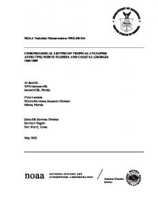
FIG. 1. Drag coefficient (C d ), and exchange coefficients (C e and C h ) at (Large and Pond) neutral conditions as calculated by the algorithm in the previous TCM3 (Wang 1999, 2001), (Modified Garratt) the formula given in Garratt (1992) with the modification in Eq. (4) that is used in the current version of the model, and by (COARE), the algorithm based on Tropical Ocean Global Atmosphere Coupled Ocean–Atmosphere Response Experiment (TOGA COARE) observations (Fairall et al. 1996).

mentation, the exchange coefficients at neutral conditions are nearly independent of the wind speed within about 25 m s 21 , but then they slightly increase with increasing wind speed as in the previous version (Fig. 1). A final, but not minor, refinement is the implementation of a time integration scheme that removes the time splitting between the model physics and model dynamics. In this new version, time tendencies at time t for zonal and meridional wind components, and temperature due to all physical processes, are evaluated at t 2 Dt. In the previous version, the model physics are included after the update of model dynamics. Therefore compared to the previous version, this new version can provide more accurate budget analysis and reduce the time splitting errors. Note that with the above refinements, the simulated tropical cyclones of the new version and the previous version are similar in general. However, for a similar minimum central surface pressure of a storm, the new version produces higher maximum surface winds than the previous version due to the use of a more selective horizontal diffusion scheme. This results in a more realistic wind–pressure relationship for the storm intensity by the new version. 3. Experimental design Eight numerical experiments (Table 2) are designed to test the effects of variations in cloud microphysics parameterization on the intensification, structure, and

DECEMBER 2002

WANG

TABLE 2. Summary of the numerical experiments. Expt CTRL WMRN NMLT HAIL NEVP CTRL E WMRN E HAIL E

Description Control experiment with standard model settings as described in section 2 As in CTRL but only the warm-rain processes are included in the cloud microphysics scheme As in CTRL but the evaporation of rain and melting of snow and graupel are excluded As in CTRL but the intercept parameters for hail (Lin et al. 1983) are used instead of those for graupel As in WMRN but the evaporation of rain is excluded As in CTRL but with an environmental flow of 10 m s21 As in WMRN but with an environmental flow of 10 m s21 As in HAIL but with an environmental flow of 10 m s21

final intensity of the model tropical cyclone. The control experiment (CTRL) is identical to the control experiment discussed in Wang (2001) except for the use of the new version of TCM3 described in the previous section. In the experiment WMRN, only warm-rain processes are retained in the cloud microphysics parameterization. In the experiment HAIL, the intercept parameters for hail (Lin et al. 1983) are used instead of those used for graupel in CTRL, as done by McCumber et al. (1991). This experiment is used to examine the effect of terminal velocity of graupel on the simulated tropical cyclone. The experiment NMLT is identical to CTRL except that the atmospheric cooling associated with evaporation of rain, and melting of snow and graupel, are excluded (but sublimation of snow and graupel and evaporation of cloud water are still included), and thus convective downdrafts would be suppressed greatly. The experiment NEVP is identical to WMRN except that the evaporation of rain is excluded; thus, the convective downdrafts are largely suppressed as is the case in NMLT. In the above five experiments, no environmental flow is considered. To examine the possible dependence of the sensitivity to cloud microphysics on movement of the model tropical cyclone, another three experiments, designated as CTRLpE, WMRNpE, and HAILpE, are designed in which a uniform easterly environmental flow of 10 m s 21 is included but with other settings being the same as those in CTRL, WMRN, and HAIL, respectively. Note that in the following discussions, when we say sensitivity to cloud microphysics parameterization, we mean the sensitivity among the first three experiments, that is, CTRL, WMRN, and HAIL, and the last three experiments, that is, CTRLpE, WMRNpE, and HAILpE, since they are standard in most cloud microphysics parameterization schemes. The changes in the cloud microphysics parameterization in all the experiments are imposed from the start of the model time integration. The initial conditions are the same as those for the control experiment given in

3025

Wang (2001, Part I) except that the initial vortex is weaker and has a maximum tangential wind of 20 m s 21 at a radius of 80 km at the surface instead of 25 m s 21 at 100 km used in Part I. In the last three experiments in Table 2, the environmental flow is in geostrophic balance initially and does not change much during the model time integration. As in Wang (2001), sea surface temperature is fixed at 298C and thus the ocean cooling due to the forcing from the model tropical cyclone was not considered. 4. The numerical results a. The evolution of storm intensity The tropical cyclone in CTRL intensified, after an initial adjustment of about 24 h, to a quasi-steady state1 after about 4 days with a lifetime low-level maximum wind speed of 79 m s 21 and a minimum central sea surface pressure of 895 hPa. This final intensity of the storm is weaker (about 15 hPa higher in the central sea surface pressure) than the maximum potential intensity (MPI) calculated from the algorithm of Holland (1997), as shown by the horizontal line in Fig. 2b. This discrepancy is largely due to the fact that in Holland’s theory, air–sea temperature difference was assumed to be 18C under the eyewall, while in our simulated tropical cyclone this difference can be as large as about 48C under the eyewall due to the cooling by the evaporation of raindrops (Wang et al. 2001). This indicates that Holland’s approach might overestimate the MPI to give lower central sea surface pressure or stronger tropical cyclones. Removing the ice-phase processes but retaining the warm-rain processes in the model cloud microphysics parameterization in WMRN provides a first-order assessment of the usefulness of simple, rain-only parameterizations on estimating tropical cyclone intensity. We see from Fig. 2 that the result is an earlier intensification than, but a similar final intensity to, that in CTRL. In this case, the cyclone reached its quasi-steady state after about 3.5 days, a half day earlier than that in the control experiment. The cyclone in the experiment HAIL with a larger terminal velocity for graupel intensified slightly earlier than, but also with a final intensity similar to, that in CTRL. These results thus indicate that the simulated tropical cyclone intensification and intensity are not quite sensitive to the details of cloud microphysics parameterizations. We will show in section 4c that the insensitivity occurred because these schemes produced similar levels of downdrafts and spiral rainbands, both being negative to rapid intensification and final intensity of the model tropical cyclones. Two extreme cases, experiments NEVP and NMLT, 1 Here and hereafter, a quasi-steady state is referred to as the state when the model tropical cyclone stops steady intensification and starts a slow variation in its intensity.

3026

MONTHLY WEATHER REVIEW

VOLUME 130

FIG. 2. Evolution of (a) the maximum wind speed (m s 21 ) at the lowest model level (about 25 m from the sea surface) and (b) the minimum central sea surface pressure (hPa) in the six experiments listed in Table 2. The horizontal line shows the MPI at the given sea surface temperature and the environmental sounding used as the initial conditions in all the numerical experiments calculated by the method of Holland (1997).

were designed to evaluate the effect of downdrafts on both the intensification and intensity of the simulated tropical cyclone. Removing the evaporation of rain in NEVP from WMRN almost removed the downdrafts in the simulated tropical cyclone; thus, both the intensification rate and final intensity of the storm were increased greatly (Fig. 2). This may be the reason why some earlier numerical models that did not include the evaporation of rain in the simple warm rain-only parameterizations produced model tropical cyclones that went straight to their local thermodynamic limit (Holland 1997). The model tropical cyclone reached its quasi-steady state in about 3 days with a final intensity (measured by the minimum central sea surface pressure) close to the MPI determined by the thermodynamic limit calculated by Holland’s (1997) approach, which did not include the effect of cooling due to evaporation of rain. The other extreme case is NMLT in which the melting of snow and graupel and the evaporation of rain were removed from CTRL. As in NEVP, the capacity to induce downdrafts in NMLT was also greatly reduced and the intensification rate and final intensity of the tropical cyclone increased dramatically (Fig. 2). The model tropical cyclone reached its quasi-steady state in about 2 days with an extremely rapid intensification. The storm

FIG. 3. Zonal–vertical cross section of mixing ratios of (a) cloud ice, (b) snow, (c) graupel, (d) cloud water, and (e) rainwater through the model tropical cyclone center after 102 h of simulation in the control experiment. Note that the unit for cloud ice, snow, and cloud water is 0.1 g kg 21 , while the unit for graupel and rain is g kg 21 . (The same units are used in the rest of the paper.)

in this case reached its final intensity even deeper (stronger) than the MPI determined by the thermodynamic approach (Holland 1997) by about 20 hPa. This extra intensity increase in NMLT compared with that in NEVP could be a result of the extra latent heat of fusion in the eyewall in the upper troposphere (see section 4d) where the warming is very effective in lowering the surface pressure (Holland 1997). b. Cloud structures of the simulated storms In the experiment CTRL with mixed-ice phase (Fig. 3), cloud ice is concentrated in the upper troposphere with a maximum at about 250 hPa in the eyewall (Fig.

DECEMBER 2002

WANG

3027

FIG. 4. Zonal–vertical cross section of mixing ratios of (a) cloud water and (b) rainwater through the model tropical cyclone center after 102 h of simulation in the warm-rain-only cloud microphysics parameterization scheme WMRN in Table 2.

3a). It is initiated through nucleation and freezing of supercooled cloud water, grows by deposition of water vapor in the eyewall, and is advected radially outward by the outflow in the upper troposphere. Snow with its maximum concentration in the 200–500-hPa layer (Fig. 3b) forms as cloud ice grows to reach a critical size (mass), and grows by both vapor deposition and collection of cloud ice and supercooled cloud water. Snow starts to convert to graupel as its size (mass) exceeds a critical value. Graupel also forms through freezing of rainwater and grows very quickly by both vapor deposition and collecting liquid and solid particles as it falls. It melts into rain in the saturated region or sublimates to water vapor in unsaturated region as it falls through the melting level. As a result, the peak mixing ratio of graupel occurs just above the melting level in the eyewall between 300 and 500 hPa (Fig. 3c). Cloud water is initiated by condensation of supersaturated water vapor; thus, a high concentration of cloud water is closely related to the outward-tilted updrafts in the eyewall (Fig. 3d). A high concentration of cloud water outside the eyewall is associated with the activity of convective rainbands with its root in the inflow boundary layer. The cloud base is mostly located between 150 and 500 m above the sea surface and even lower under the eyewall. Rainwater forms through conversion from the cloud water, and grows by collecting cloud water and by melting of both snow and graupel, and thus concentrates below the melting level (Fig. 3e). These cloud structures in our simulated tropical cyclone are all in good agreement with available observations in real tropical cyclones (Black and Hallett 1986; Houze et al. 1992; Marks and Houze 1987) and also with simulations with some other tropical cyclone models (Liu et al. 1997). With no ice phase in WMRN, the upper-level ice cloud is replaced by liquid water cloud (Fig. 4a). In this case, cloud water forms by condensation in the eyewall

FIG. 5. As in Fig. 3 but for expt HAIL in Table 2. Note that in (c) mixing ratio of hail is shown.

updrafts and is advected radially outward in the upper troposphere, producing both anvil and stratiform clouds in the upper troposphere outside the eyewall. There are also some boundary layer clouds outside the eyewall (Fig. 4a). Rainwater extends up to about 150 hPa in the eyewall and tilts outward with height, thus producing stratiform precipitation outside the eyewall (Fig. 4b). Using the parameters for hail in HAIL instead of that for graupel in CTRL reduced the concentration of the largest ice species (hail in this case) but increased the concentration of cloud ice, snow, and supercooled cloud water in the upper troposphere (Fig. 5). These cloud structures stem from the larger terminal velocity of hail than that of graupel. With a larger terminal velocity, the hail remained in the air for a shorter time period than the graupel and thus has less time to grow through deposition and by collecting cloud water, cloud ice, and snow as it falls. As a result, the amount of hail itself was greatly reduced, while the cloud ice, snow, and

3028

MONTHLY WEATHER REVIEW

VOLUME 130

FIG. 7. Zonal–vertical cross sections of model-estimated radar reflectivity (dBZ ) through the storm center in the expts (a) CTRL, (b) WMRN, (c) HAIL, and (d) NMLT after 102 h of simulation. The corresponding vertical structures of hydrometeors are shown in Figs. 3–6.

FIG. 6. As in Fig. 3 but for expt NMLT in Table 2.

cloud water were all increased remarkably (Fig. 5). This difference in vertical structure of the hydrometeors between graupel and hail regimes is in agreement with the findings of McCumber et al. (1991), who compared the ice-phase microphysical parameterization schemes in simulations of both squall- and nonsquall-type convection in the Tropics. Removing the melting of snow and graupel and the evaporation of rain in NMLT from CTRL results in quite different cloud structures (Fig. 6). In particular, because graupel descended without melting when it fell through the lower troposphere, it reached the sea surface as precipitants although the highest concentration of graupel was still located between 250 and 600 hPa. This high concentration of graupel manifests the existence of strong eyewall updrafts (not shown) and thus rapid rimming and depositional growth in the strongest storm among the first five experiments (Fig. 2). Because the melting of graupel and snow (major source for rain production) was excluded, cloud water that condensed in

the eyewall updrafts became the only source for rain. As a result, rain concentrated within the narrow eyewall region (Fig. 6e). Note that although there was weaker stratiform precipitation associated with graupel (Fig. 6c), neither downdrafts nor significant outer spiral rainbands developed (see section 4c), thus resulting in the strongest storm (Fig. 2). The difference in cloud structures discussed above is also clearly seen from the model-estimated radar reflectivity corresponding to the given hydrometeors shown in Figs. 3–6 (Fig. 7). In CTRL (Fig. 7a), the structure of the radar reflectivity is quite similar to that in the Hurricane Andrew (1992) simulated by Liu et al. (1997). Sharp vertical gradients in radar reflectivity occurred near the freezing level at about 500 hPa in the eyewall with an eye nearly free of reflectivity and some high reflectivity associated with the rainbands outside the eyewall (Fig. 7a). Anvil clouds extended outward above the eyewall in the upper troposphere. In WMRN, the high reflectivity in the eyewall penetrated into the upper troposphere with relatively less stratiform cloud outside the eyewall (Fig. 7b) than that in CTRL. Replacing the graupel by hail in HAIL produced high re-

DECEMBER 2002

WANG

flectivity below the freezing level in the eyewall, similar to that in the control experiment, but with more pronounced stratiform clouds in the mid–upper troposphere (Fig. 7c) due to the higher concentration of cloud ice and snow than that in the control experiment (Figs. 3 and 5). In NMLT with neither melting of snow and graupel nor evaporation of rain, in addition to the high radar reflectivity in the deep eyewall, there is a large area of stratiform precipitation with relatively weak reflectivity outside the eyewall (Fig. 7d), which is quite different from that in the control experiment (Fig. 7a). The reflectivity in the storm eye region indicates light precipitation associated with graupel that was detrained from the eyewall (Fig. 6c). In summary, different from the intensity discussed in section 4a, the cloud structures in the simulated tropical cyclone are quite sensitive to the parameterization of cloud microphysics in the model. The mixed-ice-phase cloud microphysics is important to realistically simulating the cloud structures in a tropical cyclone. As found by McCumber et al. (1991), the optimal mix of the bulk ice hydrometeors is cloud ice–snow–graupel for use in tropical cyclone models. c. Spiral rainbands and downdrafts Previous studies suggested that the rainbands play two roles in limiting the intensity of tropical cyclones (e.g., Barnes et al. 1983; Powell 1990a,b). First, downdrafts are initiated by the melting of snow and graupel and the evaporation of rain and usually form just inside the rainbands. These downdrafts bring dry and cold air with low equivalent potential temperature (u e ) from the midtroposphere into the inflow boundary layer. The air with low u e is advected to the core region by the boundary layer inflow and entrained into the eyewall, thus suppressing the convection in the eyewall and reducing the intensity of a tropical cyclone. In addition, the mass and moisture convergence into the rainbands plays a barrier role in reducing the boundary layer inflow toward the eyewall, reducing the mass and moisture convergence into the eyewall, the eyewall updrafts, and eyewall convection, and thus reducing the cyclone intensity. As a result, active spiral rainbands and associated strong downdrafts can be referred to as prohibiting factors to tropical cyclone intensification and intensity. In both CTRL (Fig. 8a) and HAIL (Fig. 8c), there are active spiral rainbands outside the eyewall in the simulated tropical cyclones. Downdrafts associated with these spiral rainbands and from the stratiform cloud region are responsible for the low u e in the boundary layer (Figs. 9a,c). The low u e is advected spirally into the eyewall region as seen from the superimposed streamlines given in Figs. 9a,c, suppressing the eyewall convection, and thus reducing the cyclone intensity. The cyclone in WMRN has slightly less active rainbands (Fig. 8b) and thus u e is higher in the near-core region

3029

in the boundary layer (Fig. 9b) than in either CTRL or HAIL. This may explain the earlier intensification and a slightly stronger cyclone at this time in WMRN (Figs. 2). In NMLT, although there are large areas with relatively high reflectivity in the near-core region (Fig. 8d), there are no significant downdrafts and thus the u e in the boundary layer is high even outside of the eyewall (Fig. 9d). As a result, the cyclone in NMLT is much stronger than those in the other experiments. This demonstrates that the melting of snow and graupel and evaporation of rain are both responsible for generation of downdrafts and spiral rainbands, both limiting the intensification rate and final intensity of a tropical cyclone. To further demonstrate the role of downdrafts in reducing the intensification rate of the simulated tropical cyclone, we show in Fig. 10 the percentages of area coverage of radar reflectivity greater than 30 dBZ (panel a) and u e less than 360 K (panel b) as a function of time and radius from t 5 0 to 96 h in the control experiment. Rainfall started after about 4 h of simulation (Fig. 10a) while low u e caused by downdrafts seemed to develop about 3 h later (fig. 10b). Before 20 h of simulation, the outward extension of rainfall manifests the activity of rainbands that propagated outward up to a radius of about 180 km. Accompanying the outward propagating rainbands was an outward extension of large area with low u e , indicating the existence of strong downdrafts associated with the rainbands. The high reflectivity within about 60-km radius developed after about 12 h of simulation when the rainbands that developed earlier propagated away from the inner-core region. This is followed by a gradual intensification of the model tropical cyclone. The low u e due to downdrafts continuously generated in the original rainbands seemed to have a prolonged prohibiting effect on the rapid intensification of the cyclone up to about 36 h. Although downdrafts were also generated by eyewall convection, as seen from the low u e near the eyewall in Fig. 10b, their effect is not as significant as those in the spiral rainbands, especially after the storm reached a certain intensity. This is because the relative humidity in the eyewall is higher under the eyewall than that outside the eyewall. Thus cooling due to the evaporation of rain is relatively reduced under the eyewall. In addition, although melting of snow and graupel was also occurring in the eyewall, but due to the high u e throughout the troposphere in the eyewall (Wang 2001), this melting process could not produce strong downdrafts in the eyewall, especially after the eyewall convection was fully developed. The intensification was accompanied by shrinking of the eyewall, which is visible from the inward shrinking of large percentage coverage of high reflectivity in Fig. 10a. Spiral rainbands are active throughout the simulation as seen from the high percentage of coverage of the high reflectivity outside the eyewall (Fig. 10a) and they are also responsible for the development of downdrafts outside the eyewall (Fig. 10b) even after the storm reached its quasi-steady state (not shown).

3030

MONTHLY WEATHER REVIEW

VOLUME 130

FIG. 8. Horizontal distribution of surface radar reflectivity (dBZ ) in the four experiments shown in Fig. 7 at the same given time for each experiment. The domain shown in each panel is 360 km by 360 km. Circles are in 30-km intervals from the cyclone center. (a) The line in the northeast quadrant is used in Fig. 11 for a vertical cross section to show the vertical structure of the rainbands.

The typical structure of the spiral rainbands in our simulated tropical cyclone has many similarities to those in real tropical cyclones as discussed by Barnes et al. (1983) and Powell (1990a,b). An example is provided in Fig. 11, which shows the radial–vertical structure along the line segment indicated in Fig. 8a for the control experiment after 102 h of simulation. There are two active rainbands along this radial segment. The inner one is located at about 60 km from the cyclone center (Fig. 11a) and the other one is located between 90- and 120-km radii. There is an updraft core (Fig. 11c) with large condensational heating (Fig. 11d) and a local maximum in u e within each rainband, especially for the stronger outer rainband (Figs. 11c,d). Downdrafts (Fig. 11c) occurred on both the inner and outer sides of the rainbands (Figs. 11c,d). Some of these downdrafts are penetrative and are initiated by sublimative cooling of ice species that are detrained out of the clouds, especially in the upper troposphere (Figs. 11c,d), while some of them occurred just below the melting level or in the lower boundary layer and are initiated by melting of

snow and graupel and evaporation of rain. Downdrafts originating in the middle troposphere usually bring air with low u e down into the planetary boundary layer, forming low-u e pools (Figs. 9a and 11b). Although the air with low u e in the inflow boundary layer can partially be recovered by extracting sensible and latent heat fluxes from the underlying ocean on its way to being advected to the eyewall region, u e can still be lower than that under the eyewall when the air arrives at the eyewall region (Figs. 9a and 11b) and thus suppresses the eyewall convection. This is the case especially when the rainbands are not too far from the eyewall and the associated downdrafts are strong. Strong updrafts in convective rainbands are accompanied by strong mass and moisture convergence into the rainbands in the lower troposphere, thus reducing the inflow on the inner side of the rainbands and suppressing updrafts and convection in the eyewall. This reduction of inflow is referred to as the rainband barrier effect and can be seen from the radial flow given in Fig. 11f. The inflow just inside the strong outer rainband

DECEMBER 2002

WANG

3031

FIG. 9. Equivalent potential temperature u e (K) at the lowest model level for the corresponding radar reflectivity in the four experiments shown in Fig. 8. Streamlines at the lowest model level are superimposed.

around the radius of 90–120 km is largely reduced in the lower troposphere below about 800 hPa due to the barrier effect of the rainband. The tangential flow inside the rainband is also reduced with a local minimum while it is increased outside the rainband (Fig. 11e). This means a local increase in cyclonic shear across the rainband. This is consistent with the PV concentration in the lower troposphere associated with the condensational heating in the rainband (Fig. 11d), in agreement with previous observational studies (Powell 1990a; May and Holland 1999). The above results imply that extensive stratiform clouds and the presence of strong rainbands and downdrafts have a substantial negative impact upon the intensification and the intensity that a tropical cyclone can achieve. Therefore, to accurately predict the intensity and intensity change of tropical cyclones by numerical models, the models should be able to produce realistic mesoscale features, such as the spiral rainbands and associated downdrafts and the eyewall structure of a tropical cyclone. Since the activity of the spiral rainbands and the associated downdrafts in the experiments CTRL, WMRN, and HAIL is at similar level, the difference in the final intensity of the model tropical cyclone in these

experiments is thus not significant because the thermodynamic structure of their environment and the underline sea surface temperature are the same in these experiments. d. Precipitation and vertical heating profile It is also our interests to examine the differences in the distribution and intensity of precipitation and the vertical profile of condensational heating due to variations in the details of the cloud microphysics parameterization. Since our interest is to look at the sensitivity of the simulated tropical cyclone to the details of ‘‘realistic’’ cloud microphysics parameterizations, only the precipitation and vertical profile of condensational heating in the first three experiments (Table 2) are discussed in this section. As seen from Fig. 12a, during the intensification stage, the rainfall rate under the eyewall in WMRN is the largest among the three experiments and is about 180% of that in CTRL and 135% of that in HAIL. This explains the earlier development and greater intensity of the cyclone in WMRN than that in either CTRL or HAIL during the same time period. The rainfall under the eyewall in CTRL is the smallest among

3032

MONTHLY WEATHER REVIEW

VOLUME 130

FIG. 10. Radial–time Hovmo¨ller diagram of (a) the percentage areal coverage of radar reflectivity greater than 30 dBZ and (b) that of the equivalent potential temperature less than 360 K at the lowest model level, showing the activity of rainbands and the associated downdrafts during the intensification stage between 0 and 96 h of simulation in CTRL listed in Table 2.

the three experiments, but it is relatively large outside a radius of about 70 km from the cyclone center (Fig. 12a). The latter indicates the existence of active outer spiral rainbands (see also Fig. 10), which reduces the convection in the eyewall and the intensification rate of the model cyclone, as discussed in the last subsection. During the mature stage (Fig. 12b), the relative magnitudes of rainfall rates under the eyewall in the three experiments are not changed in comparison with the intensification stage (Fig. 12a) except that the difference in magnitude becomes smaller. Note that although the intensities of the model tropical cyclones are quite similar during this time period, the rainfall rate under the eyewall differs significantly in the three experiments (Fig. 12b). This indicates that although the intensity of the model tropical cyclone is not very sensitive to the details of the cloud microphysics parameterization, the difference in rainfall can be large. For example, in the three experiments, rainfall rate under the eyewall in HAIL is about 20% larger than that in CTRL, while that in WMRN is about 40% larger than that in CTRL. However, outside the eyewall between 40- and 70-km

radii, the precipitation area in CTRL is larger than that in either WMRN or HAIL. These results are in agreement with the findings of McCumber et al. (1991), who also found that ice-free (warm rain only) cloud microphysics produced too large of a peak rainfall rate but with less extensive area coverage (see their Table 5). Consistent with the radial distribution of rainfall rate shown in Fig. 12b, the condensational heating rate in the eyewall region (between 15- and 35-km radii) is largest in WMRN but smallest in CTRL (Fig. 13a). The vertical heating profiles are similar in the three experiments although there are some slightly differences. Maximum heating in the eyewall occurred in the mid– upper troposphere (5–8 km) in the three experiments with the maximum heating level being slightly higher in both WMRN and HAIL (Fig. 13a). There is a cooling near the sea surface with a cooling rate larger than 5 K h 21 . This cooling results from evaporation of falling rain in the subcloud layer. The condensational heating within a radius of 100 km is quite similar in the three experiments except for a slightly smaller heating rate in the mid–upper troposphere in WMRN (Fig. 13b).

DECEMBER 2002

WANG

3033

FIG. 11. Vertical cross section along the line segment given in Fig. 8a, showing the vertical structure of the rainbands in the control experiment: (a) Radar reflectivity (dBZ ), (b) equivalent potential temperature (K), (c) vertical motion (m s 21 ), (d) condensational heating rate (K h 21 ), (e) tangential wind (m s 21 ), and (f ) radial wind (m s 21 ).

This can explain the similar intensity of the model tropical cyclones during this period (Fig. 2). These results therefore demonstrate that the overall vertical heating profile is not very sensitive to the details of cloud microphysics parameterization while the peak intensity and area coverage in precipitation can be very sensitive. e. Effect of an environmental flow Since the results discussed above are obtained from the numerical experiments with an environment at rest, a question arises as to whether the sensitivity will be changed if an environmental flow is considered. To answer this question, we include a uniform environmental flow of 10 m s 21 in the last three experiments (Table 2). The evolution of storm intensity in the three experiments is shown in Fig. 14. We can see that the

sensitivity is not changed in general, especially for the two cases with mixed-ice phase cloud microphysics (CTRLpE and HAILpE). The difference in storm intensity between the ice-free (WMRNpE) and mixedice phase (CTRLpE and HAILpE) becomes larger in an environmental flow than in a quiescent environment (Figs. 2 and 14). Since we have indicated that ice-free cloud microphysics seems to overestimate the storm intensity and also overpredict the rainfall rate under the eyewall, we thus intend to recommend the use of mixed-ice-phase cloud microphysics parameterization in tropical cyclone models. Therefore, our observation of the weak sensitivity of the simulated tropical cyclone intensity to the details of cloud microphysics parameterization remains unchanged and thus is little dependent on the environmental flow or the movement of the tropical cyclones.

3034

MONTHLY WEATHER REVIEW

VOLUME 130

FIG. 12. Azimuthally averaged, 6-hourly mean radial distribution of rainfall rate in CTRL, WMRN, and HAIL, (a) between 36 and 42 h and (b) between 126 and 132 h.

5. Conclusions and discussion In the most advanced simulation of tropical cyclones by numerical models, the use of explicit cloud microphysics has become increasingly attractive while cumulus convective parameterization schemes are usually bypassed at very high model resolution. However, although it has long been known that cloud microphysics can have a significant impact on the simulations of precipitation, there have been few studies so far that have investigated the effect of cloud microphysics parameterization on simulations of tropical cyclones. In this study an initial evaluation of the sensitivity of simulated tropical cyclone structure, intensification, and intensity to the choice and details of cloud microphysics parameterizations has been carried out using the tropical cyclone model TCM3 described in Part I (Wang 2001) but with several refinements. We found that intensification rate and final intensity of the simulated tropical cyclone are not quite sensitive to the cloud microphysics parameterizations in the model. This insensitivity indicates the potential advantage in using an explicit cloud microphysics scheme in tropical cyclone models to improve the intensity forecast, compared with the substantial sensitivity of simulated tropical cyclones to different cumulus parameterization schemes found in previous studies (Baik et al. 1991; Zehnder 2001). It is shown that the insensitivity stems from the similar vertical profile and magnitude in condensational heating rate, and also to the similar level of the simulated stratiform clouds and spiral rainbands and

FIG. 13. Vertical profiles of 6-hourly mean (between 126 and 132 h) condensational heating rate in CTRL, WMRN, and HAIL: (a) azimuthally averaged between 15- and 35-km radii and (b) azimuthally averaged within a radius of 100 km from the cyclone center.

the associated downdrafts by various cloud microphysics parameterizations. The melting of snow and graupel in the stratiform clouds and evaporation of rain in the subcloud layer are major processes in initiating the spiral rainbands outside the eyewall by producing strong downdrafts. Downdrafts can be generated near the lateral edges of deep cloud towers either in the eyewall or in the rainbands by the melting of ice species and the evaporation of both cloud water and raindrops being detrained from the deep clouds. We also found that the downdrafts are major prohibiting factors limiting the intensification rate and final intensity of tropical cyclones. Spiral rainbands affect the structure, intensification, and final intensity of a tropical cyclone through two major processes. On one hand, strong downdrafts associated with the rainband bring the air with low u e from the middle troposphere and thus produce cooling and drying in the inflow boundary layer. The air with low u e can be transported into the cyclone core region and entrained into the eyewall, thus suppressing the eyewall convection. On the other hand, updrafts in the spiral rainbands are accompanied by boundary layer mass and

DECEMBER 2002

3035

WANG

cyclone intensity to the cloud microphysics parameterization found in this study will be changed or not if an interactive radiation budget is included. We plan to study separately the potential feedbacks and their effects on the structure and intensity of a tropical cyclone. In addition, this study was based on a hydrostatic primitive equation model. Although details of the simulated storms could be modified if the nonhydrostatic effect is considered, the major conclusions and interpretation of the numerical results are not expected to be changed by the nonhydrostatic effect since many aspects of the simulated storms are comparable with available observations and with other simulations with nonhydrostatic models. Acknowledgments. The author is grateful to two anonymous reviewers for their constructive comments and clarifications, which helped improve the manuscript. This study has been supported in part by ONR 000-1494-1-0493, and in part by the Frontier Research System for Global Change through the International Pacific Research Center (IPRC) in the School of Ocean and Earth Science and Technology (SOEST) at the University of Hawaii. FIG. 14. As in Fig. 2 but for expts CTRLpE, WMRNpE, and HAILpE shown in Table 2.

moisture convergence into the rainbands. The convergent flow into the rainband may partially reduce the boundary layer inflow toward the eyewall, thus reducing the updrafts in the eyewall and suppressing the eyewall convection. This suggests that in order to accurately predict the intensity and intensity change of a tropical cyclone by numerical models, the models should be able to produce realistic mesoscale features, such as the spiral rainbands and associated downdrafts and the eyewall structure of a tropical cyclone. Although both intensification rate and final intensity are not sensitive to the cloud microphysics parameterizations, the cloud structures and the peak and area coverage in precipitation in the simulated tropical cyclone are quite sensitive to the details of the cloud microphysics parameterization in the model. In agreement with the findings by McCumber et al. (1991), we also found that the mixed-ice-phase cloud microphysics is important in realistically simulating the cloud structures and precipitation in a tropical cyclone. The use of cloud information from cloud microphysics can provide a physically consistent radiation budget and thus improve the accuracy of the radiative transfer (Petch 1998). Therefore, realistic simulations of cloud structures by numerical models are important because clouds can interact with radiation, thus affecting the structure and intensity of the tropical cyclone (Krishnamurti et al. 1991; Craig 1996). It is unclear at this stage whether the insensitivity of the simulated tropical

REFERENCES Baik, J.-J., M. DeMaria, and S. Raman, 1991: Tropical cyclone simulation with Betts convective adjustment scheme. Part III: Comparison with the Kuo convective parameterization. Mon. Wea. Rev., 119, 2889–2899. Barnes, G. M., E. J. Zipser, D. P. Jorgensen, and F. D. Marks Jr., 1983: Mesoscale and convective structure of a hurricane rainband. J. Atmos. Sci., 40, 2125–2137. Black, R. A., and J. Hallett, 1986: Observations of the distribution of ice in hurricanes. J. Atmos. Sci., 43, 802–822. Braun, S. A., and W.-K. Tao, 2000: Sensitivity of high-resolution simulations of Hurricane Bob (1991) to planetary boundary layer parameterizations. Mon. Wea. Rev., 128, 3941–3961. Brown, P. R. A., and H. A. Swann, 1997: Evaluation of key microphysical parameters in three-dimensional cloud-model simulations using aircraft and multiparameter radar data. Quart. J. Roy. Meteor. Soc., 123, 2245–2275. Craig, G. C., 1996: Numerical experiments on radiation and tropical cyclones. Quart. J. Roy. Meteor. Soc., 122, 415–422. DeCosmo, J., K. B. Katsaros, S. D. Smith, R. J. Anderson, W. A. Oost, K. Bumke, and H. Chadwick, 1996: Air–sea exchange of water vapor and sensible heat: The Humidity Exchange Over the Sea (HEXOS) results. J. Geophys. Res., 101 (C5), 12 001–12 016. Detering, H. W., and D. Etling, 1985: Application of the E–« turbulence model to the atmospheric boundary layer. Bound.-Layer Meteor., 33, 113–133. Fairall, C. W., E. F. Bradley, D. P. Rogers, J. B. Edson, and G. S. Young, 1996: Bulk parameterization of air–sea fluxes for Tropical Ocean Global Atmosphere Coupled Ocean Atmosphere Response Experiment. J. Geophys. Res., 101C, 3747–3764. Garratt, J. R., 1992: The Atmospheric Boundary Layer. Cambridge University Press, 316 pp. Holland, G. J., 1997: The maximum potential intensity of tropical cyclones. J. Atmos. Sci., 54, 2519–2541. Houze, R. A., F. D. Marks Jr., and R. A. Black, 1992: Dual-aircraft investigation of the inner core of the Hurricane Norbert. Part II: Mesoscale distribution of ice particles. J. Atmos. Sci., 49, 943– 962. Jones, R. W., 1980: A three-dimensional tropical cyclone model with

3036

MONTHLY WEATHER REVIEW

release of latent heat by the resolvable scales. J. Atmos. Sci., 37, 930–938. Krishnamurti, T. N., K. S. Yap, and D. K. Oosterhof, 1991: Sensitivity of tropical storm forecast to radiative destabilization. Mon. Wea. Rev., 119, 2176–2205. Large, W. G., and S. Pond, 1982: Sensible and latent heat flux measurements over the ocean. J. Phys. Oceanogr., 12, 464–482. Lin, Y.-L., R. D. Farley, and H. D. Orville, 1983: Bulk parameterization of the snow field in a cloud model. J. Climate Appl. Meteor., 22, 1065–1092. Liu, Y., D.-L. Zhang, and M. K. Yau, 1997: A multiscale numerical study of Hurricane Andrew (1992). Part I: Explicit simulation and verification. Mon. Wea. Rev., 125, 3073–3093. ——, ——, and ——, 1999: A multiscale numerical study of Hurricane Andrew (1992). Part II: Kinematics and inner-core structures. Mon. Wea. Rev., 127, 2597–2616. Lord, S. J., H. E. Willoughby, and J. M. Piotrowicz, 1984: Role of a parameterized ice-phase microphysics in an axisymmetric tropical cyclone model. J. Atmos. Sci., 41, 2836–2848. Marks, F. D., Jr., and R. A. Houze Jr., 1987: Inner core structure of Hurricane Alicia from airborne Doppler radar observations. J. Atmos. Sci., 44, 1296–1317. May, P. T., and G. J. Holland, 1999: The role of potential vorticity generation in tropical cyclone rainbands. J. Atmos. Sci., 56, 1224–1228. McCumber, M., W.-K. Tao, and J. Simpson, 1991: Comparison of ice-phase microphysical parameterization schemes using numerical simulation of tropical convection. J. Appl. Meteor., 30, 985–1004. Meyers, M. P., P. J. DeMott, and W. R. Cotton, 1992: New primary ice-nucleation parameterization in an explicit cloud model. J. Appl. Meteor., 31, 708–721. Petch, J. C., 1998: Improved radiative transfer calculations from information provided by bulk microphysical schemes. J. Atmos. Sci., 55, 1846–1858. Powell, M. D., 1990a: Boundary layer structure and dynamics in outer hurricane rainbands. Part I: Mesoscale rainfall and kinematic structure. Mon. Wea. Rev., 118, 891–917.

VOLUME 130

——, 1990b: Boundary layer structure and dynamics in outer hurricane rainbands. Part II: Downdraft modification and mixed layer recovery. Mon. Wea. Rev., 118, 918–938. Rosenthal, S. L., 1978: Numerical simulation of tropical cyclone development with latent heat release by resolvable scales. I: Model description and preliminary results. J. Atmos. Sci., 35, 258–271. Tripoli, G. J., 1992: An explicit three-dimensional nonhydrostatic numerical simulation of a tropical cyclone. Meteor. Atmos. Phys., 49, 229–254. Wang, Y., 1999: A triply nested movable mesh tropical cyclone model—TCM3. BMRC Research Rep. 74, 81 pp. [Available from Bureau of Meteorology Research Centre, Melbourne, Victoria 3001, Australia.] ——, 2001: An explicit simulation of tropical cyclones with a triply nested movable mesh primitive equation model—TCM3. Part I: Description of the model and control experiment. Mon. Wea. Rev., 129, 1270–1294. ——, J. D. Kepert, and G. J. Holland, 2001: The effect of sea spray evaporation on tropical cyclone boundary layer structure and intensity. Mon. Wea. Rev., 129, 2481–2500. Willoughby, H. E., H.-L. Jin, S. J. Lord, and J. M. Piotrowicz, 1984: Hurricane structure and evolution as simulated by an axisymmetric, nonhydrostatic numerical model. J. Atmos. Sci., 41, 1169–1186. Yamasaki, M., 1977: A preliminary experiment of the tropical cyclone without parameterizing the effect of cumulus convection. J. Meteor. Soc. Japan, 55, 11–30. Zehnder, J. A., 2001: A comparison of convergence- and surfaceflux-based convective parameterizations with applications to tropical cyclogenesis. J. Atmos. Sci., 58, 283–301. Zhang, D.-L., 1989: The effect of parameterized ice microphysics on the simulation of vortex circulation with a mesoscale hydrostatic model. Tellus, 41A, 447–449. ——, E.-Y. Hsie, and M. W. Moncrieff, 1988: A comparison of explicit and implicit predictions of convective and stratiform precipitating weather systems with a meso-beta-scale numerical model. Quart. J. Roy. Meteor. Soc., 114, 31–60.