Hindawi Publishing Corporation Mathematical Problems in Engineering Volume 2016, Article ID 3763512, 13 pages http://dx.doi.org/10.1155/2016/3763512
Research Article An Extended Genetic Algorithm for Distributed Integration of Fuzzy Process Planning and Scheduling Shuai Zhang, Zhinan Yu, Wenyu Zhang, Dejian Yu, and Yangbing Xu School of Information, Zhejiang University of Finance and Economics, No. 18 Xueyuan Street, Xiasha, Hangzhou 310018, China Correspondence should be addressed to Zhinan Yu;
[email protected] Received 23 July 2015; Accepted 14 March 2016 Academic Editor: David Bigaud Copyright © 2016 Shuai Zhang et al. This is an open access article distributed under the Creative Commons Attribution License, which permits unrestricted use, distribution, and reproduction in any medium, provided the original work is properly cited. The distributed integration of process planning and scheduling (DIPPS) aims to simultaneously arrange the two most important manufacturing stages, process planning and scheduling, in a distributed manufacturing environment. Meanwhile, considering its advantage corresponding to actual situation, the triangle fuzzy number (TFN) is adopted in DIPPS to represent the machine processing and transportation time. In order to solve this problem and obtain the optimal or near-optimal solution, an extended genetic algorithm (EGA) with innovative three-class encoding method, improved crossover, and mutation strategies is proposed. Furthermore, a local enhancement strategy featuring machine replacement and order exchange is also added to strengthen the local search capability on the basic process of genetic algorithm. Through the verification of experiment, EGA achieves satisfactory results all in a very short period of time and demonstrates its powerful performance in dealing with the distributed integration of fuzzy process planning and scheduling (DIFPPS).
1. Introduction Nowadays in manufacturing fields, there are desperate needs for not only the integration of process planning and scheduling but also distributed manufacturing. On the one hand, although the conventional job shop scheduling problem (JSSP) is still a hotspot in the studies of manufacturing researchers and has great potential to make progress, its separation from process planning inevitably obstructs the improvement of manufacturing efficiency and disables it in tackling complicated manufacturing environment [1]; on the other hand, the distribution feature of resources such as raw materials, manpower, and technologies propels the enterprise to operate in a more decentralized way and has gradually drawn the attention of many researchers [2–4]. Besides these two concerns, there is also an urge to represent the processing time in manufacturing with fuzzy values. For instance, fuzzy job shop scheduling problem has become the main topic of production scheduling [5]. Due to the unpredictable conditions in realistic manufacturing and the different proficiency among manual workers, the processing time in manufacturing is variable in a certain
range. However, in the traditional research, it is fixed to a precise value to facilitate the calculation. To a certain extent, the fixed value loses the flexibility and definitely cannot accord with the practice. Under these circumstances, the distributed integration of processing planning and scheduling (DIPPS) is proposed first. For one thing, the DIPPS is on the basis of the integrated processing planning and scheduling (IPPS) which overcomes the deficiency of JSSP in integration; for another, it features distribution manufacturing to conform to the realistic manufacturing environment. In addition, considering the necessity of the fuzzy feature in the manufacturing and the distribution feature in the DIPPS, the fuzzy processing time and fuzzy transportation time are both introduced to replace the traditional fixed values and become an integral part of the whole model. On the basis of the several enhanced parts, the distributed integration of fuzzy process planning and scheduling (DIFPPS) is thus formulated. In order to solve this problem effectively, we construct an upgraded genetic algorithm (EGA) with local enhancement strategy. The EGA has three-class chromosome to fully encode the complex information of
2 DIFPPS, and it gets improved in both crossover and mutation strategies to reinforce the global exploration capability. Also, the local enhancement strategy is equipped in EGA to strengthen its local exploration capability by replacing the processing machines with more efficient ones and exchanging the processing order of some specific operations. The rest of the paper is arranged as follows: in Section 2, we review the related work addressing IPPS and fuzzy processing time in manufacturing; in Section 3, the DIFPPS model is proposed, and the creative EGA is constructed to deal with it; in Section 4, a two-part experiment with a case study and several comparisons is conducted to demonstrate the capability of EGA in solving DIFPPS; in Section 5, we draw our conclusion.
2. Related Work In this paper, we mostly focus on formulating and solving the distributed IPPS model with fuzzy processing and fuzzy transportation time, that is, DIFPPS. In this case, the related work is divided into two parts: one is the related work in dealing with IPPS; and the other is the implementation of fuzzy theories in manufacturing. In these two parts, we mainly discuss the application of GA and its related algorithms. 2.1. IPPS Related Work. By simultaneously arranging the process planning and scheduling, IPPS overcomes the scheduling-only deficiency of traditional JSSP and gradually inspires researchers to find the optimal or near-optimal solution with the assistance of various evolutionary algorithms. Mostly, genetic algorithm (GA) is a popular algorithm in tackling IPPS. For example, Shao et al. [6] adopted a modified GA-based approach by improving the genetic representations and operator schemes to solve IPPS. Li et al. [7] made the algorithm closer to the biological evolution by adding a learning operator to GA to record a certain amount of better solutions in the iterations. Zhang and Wong [8] constructed an object-coding GA with inferior selection and population degeneration mechanisms to strengthen the global exploration capability in dealing with IPPS. In order to further enhance the exploration capability, some other methods are also combined with GA to construct hybrid algorithms. For instance, Li et al. [9] combined GA with a local search strategy, and Yu et al. [10] used an additional particle swarm optimization to select the appropriate machines in the scheduling part. These combinations prevented GA from falling into local optima and have achieved better outcomes in the experiments than GA-only strategies. Besides the above work that is based on GA, quite a number of researchers also adopted other evolutionary algorithms, such as simulated annealing algorithm [11], imperialist competitive algorithm [12], and ant colony algorithm [13], to deal with IPPS. In the experiment and case studies, they all demonstrated their outstanding performance. However, despite their competence in solving IPPS, these algorithms still fall short of handling DIPPS due to the more complex information accompanying the distributed manufacturing.
Mathematical Problems in Engineering 2.2. Fuzzy Processing Time in Manufacturing. The theory of fuzzy sets is first introduced by Zadeh [14] and then gets improved and popular in a variety of areas. In the manufacturing field, Sakawa and Kubota [15, 16] were among those who first proposed the fuzzy job shop scheduling problem (fJSSP) in which the triangular fuzzy number (TFN) is applied to represent the fuzzy processing time and fuzzy due date. In their work, the corresponding genetic algorithms are enhanced and achieved desirable results in solving the fJSSP. After the initial exploration, a number of researchers put their efforts in the fJSSP. Lei [5, 17, 18] tried not only a Pareto archive particle swarm optimization but also a random key scheduling algorithm which used a random key representation and the extended version of the first decoding to figure out an optimal solution for fJSSP. Niu et al. [19] redefined and modified the particle swarm optimization by introducing genetic operators to update the particles and then applied this algorithm to the fJSSP. Hu et al. [20] constructed a modified differential evolution algorithm for fJSSP after proposing the ranking concept among fuzzy numbers and several novel objective functions. Li and Pan [21] combined Tabu search with the particle swarm optimization in order to promote the latter one’s local search. Moreover, the flexible job shop scheduling problem (FJSSP) which is more complicated than traditional JSSP in allowing an operation to be processed on any of the machines in a corresponding set along different routes is gradually equipped with fuzzy processing time [22]. To tackle the fuzzy flexible job shop scheduling problem (fFJSSP), Lei and Guo [23] proposed a swarm-based neighborhood search algorithm, in which they implemented a novel representation, two swaps, and insertion. Wang et al. [24] used a hybrid artificial bee colony algorithm with variable neighborhood search-based local search to enhance local exploitation in search of the optimal solution. Also, Palacios et al. [25] implemented two new neighborhood structures for the local search and proposed a genetic Tuba search for the fFJSSP. And Xu et al. [22] equipped a novel teaching-learning search mechanism with special local search operators in the solution-exploring procedure. Furthermore, there are also some work focused on some congeneric NP-hard problems such as flow shop scheduling [26, 27] and the general formulated group shop scheduling [28] with fuzzy processing time. However, rare work has been done to discuss the fuzzy processing time in IPPS or even DIFPPS environment.
3. An EGA for the DIFPPS 3.1. Problem Definition and Representation. On the basis of the definition of IPPS problem, the DIPPS problem discussed in this paper is generalized as follows: given 𝑁 independent jobs and 𝑀 geographically distributed manufacturing cells (MCs), where each possesses 𝑈 machines and owns full capability to process every given job, determine the specific MC, manufacturing plan, and schedule for each job in consideration of the constraints and objective. Specifically, due to the diversity of equipment among different MCs, the optional plans and schedules for the same job are also
Mathematical Problems in Engineering B
3
B
B
B
B
B
1 OR1
1 OR1
1
OR1 1
1 2 OR2 5
6
3
6
4 7
8
OR2
2 OR1 OR2
3
4
2
1
OR1
6
3 OR2 4
3
OR2
OR2
8 5
7
5 7
2
2
3
4
5
7 4
5
OR2
6 6
8
9
7
2 OR1
OR2
3 5
6
8
9
4 7
9
8
10
9
8
C
C
C
C
C
C
Job 1
Job 2
Job 3
Job 1
Job 2
Job 3
MC 1 (a)
(b)
MC 2 (c)
(d)
(e)
(f)
Figure 1: The network representation for jobs (Job 1–Job 3).
different among MCs. Meanwhile, jobs are delivered to a central warehouse once they are completely manufactured in certain MCs. Although there exist a variety of flexibilities in the manufacturing process [29, 30], processing flexibility that indicates the operation replaceability for the same feature in the job and operation flexibility that indicates the machine replaceability for the same operation are the major flexibilities adopted in the DIPPS problem. To represent the flexible plans and schedules for different jobs in each MC, the network that was introduced by Ho and Moodie [31] is applied as an example with two MCs and three jobs. In a network graph (Figure 1), there are three node types in the network: starting node, intermediate node, and ending node [30]. The starting node and ending node labeled “B” and “C” are dummy nodes that denote the beginning and completion of a job, while the intermediate nodes labeled numbers indicate the specific operations with alternative machines that may be done in the processing procedure. From the beginning to the completion node, the arrows connecting the nodes represent the precedence of operations [31]. Besides, the OR-links joining the arrows indicate the processing flexibility. If the links following a node are connected by an “OR” symbol, we only need to traverse one of them [31]. Thus, a job processing procedure is perfectly illustrated by a network. In Figure 1, six networks exhibit the flexible plans and schedules of three jobs in two MCs, respectively.
right represent the minimum value, the most possible value, and the maximum value, respectively. Here, several basic rules in TFN that help to achieve the necessary calculations are displayed below. Addition Rule. The addition of two TFNs is calculated as ̃+𝑊 ̃ = (V1 + 𝑤1 , V2 + 𝑤2 , V3 + 𝑤3 ) . 𝑉
Ranking Rule. Three criteria used in [18, 22, 23] are adopted to rank between two TFNs. (a) First criterion: the TFN that has higher value of (V1 + 2V2 + V3 )/4 (or (𝑤1 + 2𝑤2 + 𝑤3 )/4) ranks higher. (b) Second criterion: if two TFNs have the same result in the first criterion, then the TFN that has higher value of V2 (or 𝑤2 ) ranks higher. (c) Third criterion: if two TFNs have the same result in both first and second criteria, then the TFN that has higher value of V3 − V1 (or 𝑤3 − 𝑤1 ) ranks higher. By this means, the order of priority of all the TFNs can be figured out. Max Rule. The max of two TFNs is calculated by the rule proposed by Lei [18] as If
3.2. Fuzzy Processing Time and Fuzzy Transportation Time. ̃ = (V1 , V2 , V3 ) and Take two triangle fuzzy numbers (TFNs) 𝑉 ̃ = (𝑤1 , 𝑤2 , 𝑤3 ) as an example; three numbers from left to 𝑊
(1)
̃ > 𝑊, ̃ 𝑉
̃∨𝑊 ̃ = 𝑉; ̃ then 𝑉 ̃∨𝑊 ̃ = 𝑊. ̃ else 𝑉
(2)
4
Mathematical Problems in Engineering
Compared with other methods [15, 16], the max rule ̃∨𝑊 ̃ and applied here guarantees the triangular feature of 𝑉 makes the schedule building procedure simple [23]. 3.3. DIFPPS Problem with Fuzzy Processing and Transportation Time. Compared to the DIPPS problem we defined ̃ 𝑚,𝑛,𝑙,𝑗,𝑢 = in Section 3.1, DIFPPS problem adopts TFN 𝑃 1 2 3 (𝑝𝑚,𝑛,𝑙,𝑗,𝑢 , 𝑝𝑚,𝑛,𝑙,𝑗,𝑢 , 𝑝𝑚,𝑛,𝑙,𝑗,𝑢 ) to represent the processing time of 𝑗th operation in the plan 𝑙 of job 𝑛 that is processed by ̃ 𝑚,𝑛 = (𝑡1 , 𝑡2 , 𝑡3 ) is used to machine 𝑢 in MC 𝑚; and 𝑇 𝑚,𝑛 𝑚,𝑛 𝑚,𝑛 represent the transportation time of job 𝑛 from MC 𝑚 to the warehouse. Table 1 exhibits the alternative machines and corresponding processing time for each operation in Figure 1, while Table 2 exhibits the fuzzy transportation time for each job from a specific MC to the warehouse. To measure the superiority of plan and schedule while specifying the model, an objective and several constraints are formulated. Firstly, the corresponding notations are expounded as follows:
𝑆̃𝑚,𝑛,𝑙 ,𝑗 ,𝑢 : the starting time of any other operation processed on the same machine of 𝑂𝑚,𝑛,𝑙,𝑗,𝑢 . 𝑆̃𝑚,𝑛,𝑙,(𝑗+1),𝑢 : the starting time of the next operation of 𝑂𝑚,𝑛,𝑙,𝑗,𝑢 in the same job. ̃𝑚,𝑛,𝑙,𝑗,𝑢 : the completion time of 𝑂𝑚,𝑛,𝑙,𝑗,𝑢 . 𝐶 ̃𝑚,𝑛,𝑙 ,𝑗 ,𝑢 : the completion time of 𝑂𝑚,𝑛,𝑙 ,𝑗 ,𝑢 . 𝐶 ̃ 𝑚,𝑛 : the completion time of job 𝑛 in MC 𝑚. 𝐸 𝑋𝑚,𝑛 : if job 𝑛 is assigned to MC 𝑚, set to 1; if not, set to 0. ̃ Objective. Minimize the final completion time (FCT) 𝐹, which is the time cost from the beginning of the first job’s manufacturing to the completion of last job’s transportation: 𝑀
̃ 𝑚,𝑛 )} . ̃ 𝑚,𝑛 + 𝑇 ̃ = max { ∑ 𝑋𝑚,𝑛 ⋅ (𝐸 𝐹 𝑛∈[1,𝑁]
𝑀: the quantity of MCs.
(3)
𝑚=1
𝑁: the quantity of jobs. 𝐿 𝑚,𝑛 : the quantity of plans of job 𝑛 in MC 𝑚. 𝐽𝑚,𝑛,𝑙 : the quantity of operations of plan 𝑙 of job 𝑛 in MC 𝑚. 𝑈𝑚 : the quantity of machines in MC 𝑚.
𝑀
∑ 𝑋𝑚,𝑛 = 1 𝑛 ∈ [1, 𝑁] .
(4)
𝑚=1
𝑂𝑚,𝑛,𝑙,𝑗,𝑢 : the 𝑗th operation of plan 𝑙 of job 𝑛 processed by machine 𝑢 in MC 𝑚. 𝑆̃𝑚,𝑛,𝑙,𝑗,𝑢 : the starting time of 𝑂𝑚,𝑛,𝑙,𝑗,𝑢 . ̃𝑚,𝑛,𝑙,𝑗,𝑢 = 𝑆̃𝑚,𝑛,𝑙,𝑗,𝑢 + 𝑃 ̃ 𝑚,𝑛,𝑙,𝑗,𝑢 𝐶
Constraint 1. One job can only be assigned to one MC:
Constraint 2. No interruption is allowed during the processing of an operation:
𝑚 ∈ [1, 𝑀] , 𝑛 ∈ [1, 𝑁] , 𝑙 ∈ [1, 𝐿 𝑚,𝑛 ] , 𝑗 ∈ [1, 𝐽𝑚,𝑛,𝑙 ] , 𝑢 ∈ [1, 𝑈𝑚 ] .
(5)
Constraint 3. One machine can only process one job at 𝑠 same time:
If
𝑆̃𝑚,𝑛,𝑙 ,𝑗 ,𝑢 < 𝑆̃𝑚,𝑛,𝑙,𝑗,𝑢 ,
̃𝑚,𝑛,𝑙 ,𝑗 ,𝑢 < 𝑆̃𝑚,𝑛,𝑙,𝑗,𝑢 ; then 𝐶
(6)
̃𝑚,𝑛,𝑙,𝑗,𝑢 else 𝑆̃𝑚,𝑛,𝑙 ,𝑗 ,𝑢 > 𝐶 𝑚 ∈ [1, 𝑀] , 𝑛 ∈ [1, 𝑁] , 𝑙, 𝑙 ∈ [1, 𝐿 𝑚,𝑛 ] , 𝑗, 𝑗 ∈ [1, 𝐽𝑚,𝑛,𝑙 ] , 𝑢 ∈ [1, 𝑈𝑚 ] .
Constraint 4. The operating order of two operations in the same job cannot be altered:
̃𝑚,𝑛,𝑙,𝑗,𝑢 ∨ 𝑆̃𝑚,𝑛,𝑙,(𝑗+1),𝑢 = 𝑆̃𝑚,𝑛,𝑙,(𝑗+1),𝑢 𝐶
𝑚 ∈ [1, 𝑀] , 𝑛 ∈ [1, 𝑁] , 𝑙 ∈ [1, 𝐿 𝑚,𝑛 ] , 𝑗 ∈ [1, 𝐽𝑚,𝑛,𝑙 − 1] , 𝑢, 𝑢 ∈ [1, 𝑈𝑚 ] .
(7)
3
2
1
Job
1 2 3 4 5 6 7 8 9 1 2 3 4 5 6 7 8 1 2 3 4 5 6 7 8 9 10
Operation
(20, 24, 30)
(17, 27, 33)
(26, 27, 35)
(8, 15, 21) (13, 17, 26) (15, 17, 24) (19, 25, 29) (14, 20, 27) (13, 19, 27) (11, 15, 19)
(25, 31, 37) (26, 31, 39)
(5, 9, 15) (8, 12, 17)
(5, 12, 20) (27, 35, 40) (10, 16, 20)
1
(7, 18, 33) (20, 25, 27) (29, 31, 36) (14, 16, 25) (11, 15, 26)
(10, 19, 31) (24, 32, 37) (9, 18, 25)
(20, 25, 29) (18, 24, 33)
(24, 27, 32) (13, 17, 25) (17, 24, 33) (19, 23, 29) (17, 23, 25) (21, 25, 27) (34, 37, 38)
(16, 21, 27) (12, 15, 17)
Machine in MC 1 3 (24, 30, 35) (15, 21, 32) (10, 15, 23)
(8, 14, 21) (17, 26, 33)
(27, 35, 41) (27, 34, 39)
(17, 24, 28)
(12, 16, 25)
(11, 15, 24) (19, 23, 25) (21, 33, 45) (28, 36, 45)
(7, 13, 20)
2 (12, 18, 27) (10, 18, 24)
(19, 26, 33)
(16, 25, 30)
(29, 31, 38) (29, 35, 43) (27, 32, 35) (27, 32, 34) (12, 18, 23) (21, 25, 29) (17, 22, 28) (10, 17, 26)
(23, 29, 34)
(21, 29, 33) (24, 31, 35) (14, 19, 31) (19, 26, 31) (18, 30, 41) (15, 26, 33)
(16, 22, 27) (14, 17, 23)
4 (14, 26, 36)
(19, 28, 31) (29, 34, 38) (9, 13, 22) (22, 27, 33) (17, 23, 29)
(20, 26, 29) (26, 31, 34)
(30, 34, 39) (26, 33, 37)
(28, 32, 35) (30, 34, 37) (28, 32, 35) (26, 32, 37)
(29, 32, 37) (22, 25, 26) (27, 30, 31) (17, 20, 26)
5
(22, 27, 33)
(30, 33, 37) (25, 33, 39)
(22, 29, 35)
(19, 26, 31) (9, 14, 20)
(27, 36, 44)
(6, 14, 28) (10, 17, 26)
(9, 16, 26)
(10, 17, 23) (24, 25, 37) (16, 28, 37)
1 (25, 34, 39)
Table 1: The processing time for each operation (Job 1–Job 3).
(28, 36, 43) (11, 15, 22) (18, 23, 31) (27, 31, 35)
(19, 25, 34) (19, 24, 28)
(12, 16, 21) (27, 33, 39)
(26, 30, 34) (22, 30, 40)
(12, 19, 23) (15, 19, 27) (22, 31, 40)
(18, 23, 32)
2 (11, 16, 28) (17, 19, 25)
(16, 18, 24)
(28, 32, 37) (18, 24, 32) (19, 25, 30) (20, 24, 27) (20, 23, 27) (9, 14, 25)
(24, 27, 33) (10, 19, 27) (18, 23, 27)
(19, 28, 33) (6, 15, 29)
(28, 33, 39) (25, 31, 43) (24, 35, 39) (19, 26, 35)
Machine in MC 2 3
(17, 24, 31) (16, 24, 32) (25, 30, 33)
(11, 14, 18)
(22, 27, 30) (14, 19, 23)
(14, 20, 28) (10, 15, 22) (11, 17, 22) (6, 10, 19) (20, 24, 31) (27, 33, 35) (19, 25, 33) (31, 34, 37)
(25, 33, 41)
4 (18, 25, 29) (29, 34, 38) (6, 11, 19) (33, 40, 43)
(28, 34, 41) (7, 15, 23)
(11, 15, 20)
(34, 38, 43) (21, 25, 31) (8, 15, 22) (12, 17, 25) (22, 26, 30)
(10, 19, 25)
(14, 21, 28) (24, 29, 33) (19, 24, 31)
(12, 17, 23) (11, 18, 25) (25, 31, 36) (12, 17, 25)
(20, 22, 31)
5 (26, 31, 39) (11, 36, 45)
Mathematical Problems in Engineering 5
6
Mathematical Problems in Engineering Table 2: The fuzzy transportation time (Job 1–Job 3).
MC MC 1 MC 2
Job 1 (21, 33, 40) (15, 19, 27)
Job Job 2 (13, 20, 30) (25, 30, 34)
Job 3 (17, 19, 23) (26, 33, 35)
3.4. An Extended Genetic Algorithm 3.4.1. Encoding and Decoding. A three-class encoding method is implemented to construct chromosomes, each of which contains all the required information. In this case, the gene (Figure 2) is thus divided into three correlative sections with different classes. The first section from the left, that is, the first class, is used to encode the distribution information for each job. From left to right, genes in this section store the selected MC numbers for jobs in sequence. In Figure 2, this section has numbers “1,” “2,” and “1,” which means Jobs 1, 2, and 3, are processed in MCs 1, 2, and 1, respectively. In the second section, that is, the second class, each gene deposits the planning information for each job in sequence. For a specific job, we first rank its OR-links in the network graph. Take Figure 1 for example, every OR-link is marked with different numbers to identify its ranking: “OR1” means the OR-link is ranked first, and “OR2” means it is ranked second. Then, we determine the link information: the left link in an “OR-link” is labeled as “1,” while the right link is labeled as “2.” On this basis, each gene in the second part is divided into several rows. And from top to bottom, each row contains one OR-link’s link information. For example, in Figure 2, the corresponding gene of Job 1 in the seconding part contains “2” and “1” from top to bottom, which means the process plan of Job 1 in MC 1 goes right in the “OR1” and goes left in “OR2.” However, considering that there is no more “OR-link” after choosing the right link in “OR1,” the link information of “OR2” is thus neglected, and the chosen plan of Job 1 is 1-2-57-9 according to Figure 1(a). Once the first and second sections are settled down, the third section is employed to decide the schedules for jobs. In this section, each job’s operations in schedules are placed in sequence from left to right while blended together with other jobs’ operations. The gene number each job occupies is as much as the operation number in its longest plan among all MCs. Thus, the total gene number in this section is the addition of all jobs’ occupied genes. For each gene, it stands for an operation and has two labeled numbers to identify its corresponding job and chosen machine. Because the alternative machines for one operation show no regularity, we resequence them from “1” for each operation and use the resequenced machine number in the gene. For example, the first gene of the third part in Figure 2 belongs to Job 1’s first operation, and the resequenced machine number “3” means this operation chooses the third alternative machine, that is, Machine 5, according to Figure 1(a) and Table 1. By means of the above encoding method, all the planning and scheduling information can be inserted into a chromosome.
In the traditional IPPS and JSSP problem, the active schedule [32] that ensures the reasonability and optimum in real execution is always adopted to decode the chromosome. Here, because of the feature of fuzzy processing time, a leftshift scheme is implemented in this paper to improve the schedule in decoding by shifting the operations to the left as compact as possible [22, 24, 33]. 3.4.2. Crossover. In this procedure, we implement a binary mask in helping decide the crossover scheme for two parent chromosomes (Figure 3). This binary mask is as long as the job number, and each part of it represents the corresponding scheme for a certain job. When the randomly generated binary numbers are settled in all parts from left to right, the crossover scheme is also settled for Job 1 to 𝑁. Specifically, for those jobs who are assigned “1” in the corresponding parts of the mask, all their planning and scheduling information in Parent A (B) is directly duplicated to the same positions of Offspring A (B); while for those jobs who are assigned “0,” their information in Parent A (B) is duplicated to fill the bank positions in sequence. However, because the crossover needs the participation of two parents, the all “1” or all “0” situation in binary mask is not allowed. 3.4.3. Mutation. To mutate the chromosome, we also create a mask so as to improve the flexibility in mutation (Figure 4). The mutation mask consists of three parts for three different functions. The first part in the mask helps to decide which job information to mutate. In this case, the number in the first part can randomly choose among 1, 2, and 3 to represent Job 1, Job 2, and Job 3, respectively. After appointing a specific job, the number in the second part helps to determine the mutation range: “1” means the mutation only acts on the third section of the chromosome by randomly changing the machine number of the assigned job; “2” means the mutation also randomly changes the job’s plan in second section; and “3” means the mutation extends its action range to the first section by randomly changing the MC number. The third part of the mask is a randomly generated binary number. If it is “1,” then the assigned job’s genes in the third section of chromosome will change positions with its former job (Job 1’s former job is Job 4); and if it is “0,” do nothing. However, when Job A and Job B have 𝑎 and 𝑏 genes in the third section, respectively, and 𝑎 < 𝑏, then the change action will only act on the former 𝑎 genes of Job B without disturbing the last 𝑏−𝑎 genes. According to the binary mask in Figure 4, Job 1’s MC, plan, and processing machines are all mutated, and then its operation genes are replaced with those of Job 3’s. 3.4.4. Local Enhancement Strategy. Because of the big solution space of DIFPPS and the complexity of fuzzy intervals, it is hard to exploit a globally optimal method through the conventional procedures of genetic algorithm. So, we add a local enhancement strategy in this paper to assist the genetic algorithm. The idea of this strategy is inspired by the local search used in Xu et al. [22], and it is operated through the following two parts.
Mathematical Problems in Engineering
2
1
Operation
Plan
MC number 1
7
Resequenced machine number
2
1
2
1
2
2
[1, 3] [3, 4] [1, 2] [2, 1] [3, 3] [2, 1] [1, 2] [2, 3] [3, 2] [2, 2] [3, 3] [1, 1] [3, 4] [1, 4] [2, 1] Job number
First section
Second section
Third section
Figure 2: Chromosome representation. Mask
1
0
1
Parent A
1
2
1
Offspring A
1
2
1
Parent B
2
2
1
Offspring B
2
2
1
Parent A
1
2
1
2
1
2
1
2
2
2
2
2
1
2
2
1
2
2
2
2
1
1
1
2
2
2
1
2
1
2
1
2
2
[1, 3] [3, 4] [1, 2] [2, 1] [3, 3] [2, 1] [1, 2] [2, 3] [3, 2] [2, 2] [3, 3] [1, 1] [3, 4] [1, 4] [2, 1]
[1, 3] [3, 4] [1, 2] [2, 2] [3, 3] [2, 4] [1, 2] [2, 1] [3, 2] [2, 3] [3, 3] [1, 1] [3, 4] [1, 4] [2, 1]
[3, 2] [1, 3] [3, 4] [2, 2] [1, 3] [3, 1] [1, 1] [2, 4] [3, 2] [2, 1] [1, 2] [2, 3] [1, 1] [2, 1] [3, 4]
[3, 2] [1, 3] [3, 4] [2, 1] [1, 3] [3, 1] [1, 1] [2, 1] [3, 2] [2, 3] [1, 2] [2, 2] [1, 1] [2, 1] [3, 4]
[1, 3] [3, 4] [1, 2] [2, 1] [3, 3] [2, 1] [1, 2] [2, 3] [3, 2] [2, 2] [3, 3] [1, 1] [3, 4] [1, 4] [2, 1]
Figure 3: Crossover strategy.
(1) Machine Replacement. The machine replacement is expected to reduce the FCT by minimizing the makespan in each MC through machine alteration. First, we need to find out the jobs that have the maximal makespan in every MC and locate the corresponding operations in the third section of the chromosome. Then, replace each selected operation’s machine with the least time-costing machine the operation can choose. And if the previous machine is already the most efficient one, keep it unchanged. For example, in Figure 5, processing machines of Job 3’s operations are replaced with the other ones. However, considering that the 2nd, 4th, and 5th operations of the job have already chosen the best machine, the replacement is only conducted at the 1st and 3rd operations. (2) Order Exchange. In this step, two operations’ positions will be exchanged in order to strengthen the flexibility of the schedule and the diversity of the generation. Given two operations A and B, only if the following two conditions are all satisfied, the order exchange of A and B can take place. To be specific, these two conditions are set to prevent the illegal chromosome after the order exchange: (a) A and B belong to different jobs but are processed on the same machine in a MC.
(b) Any intermediate operations between A and B in the third section of the chromosome do not belong to the jobs that A or B belongs to. Once these two operations’ positions are exchanged, they are fixed and cannot be exchanged again. And the order exchange ends after all the possible exchanges are executed. For example, in Figure 6, the 5th and 6th operations (both processed on Machine 5 in MC 2) and the 9th and 10th operations (both processed on Machine 3 in MC 2) will exchange their positions. Through machine replacement and order exchange, the chromosome is restructured to a renewed one. However, because the renewed chromosome may degenerate, that is, having longer FCT than the original one, we determine that the chromosome with better performance will be reserved, while the other one will be abandoned.
4. Experiment The experiment is divided into two parts to demonstrate the exploration capability of EGA in managing DIFPPS problem. In the first part, EGA is applied to a case with six jobs and two MCs, while in the second part, a GA used to be applied in IPPS is adapted to deal with DIFPPS and
8
Mathematical Problems in Engineering Mask 1
1
3
1
2
1
2
2
1
2
2
1
2
2
2
1
2
2
1
2
2
2
2
2
1
2
2
2
2
2
[1, 3] [3, 4] [1, 2] [2, 2] [3, 3] [2, 4] [1, 2] [2, 1] [3, 2] [2, 3] [3, 3] [1, 1] [3, 4] [1, 4] [2, 1]
[1, 1] [3, 4] [1, 3] [2, 2] [3, 3] [2, 4] [1, 3] [2, 1] [3, 2] [2, 3] [3, 3] [1, 4] [3, 4] [1, 2] [2, 1]
[3, 4] [1, 1] [3, 3] [2, 2] [1, 3] [2, 4] [3, 2] [2, 1] [1, 3] [2, 3] [1, 4] [3, 3] [1, 2] [3, 4] [2, 1]
Figure 4: Mutation strategy.
2
2
1
2
2
1
1
2
2
2
2
2
1
2
2
2
2
2
[3, 4] [1, 1] [3, 3] [2, 2] [1, 3] [2, 4] [3, 2] [2, 1] [1, 3] [2, 3] [1, 4] [3, 3] [1, 2] [3, 4] [2, 1]
[3, 1] [1, 1] [3, 3] [2, 2] [1, 3] [2, 4] [3, 3] [2, 1] [1, 3] [2, 3] [1, 4] [3, 3] [1, 2] [3, 4] [2, 1]
Figure 5: Machine replacement.
2
2
1
2
2
1
1
2
2
2
2
2
1
2
2
2
2
2
[3, 4] [1, 1] [3, 3] [2, 2] [1, 3] [2, 4] [3, 2] [2, 1] [1, 3] [2, 3] [1, 4] [3, 3] [1, 2] [3, 4] [2, 1]
[3, 4] [1, 1] [3, 3] [2, 2] [2, 4] [1, 3] [3, 2] [2, 1] [2, 3] [1, 3] [1, 4] [3, 3] [1, 2] [3, 4] [2, 1]
Figure 6: Order exchange. B
B
OR1
OR1
1
1
2
2
OR2 4
3 OR2
6 7
8
9
B
B
1
1 OR1
1
1 OR1
3
OR3 7
5
6
8
4 OR2
4 OR2 6
5
3
2
OR1
OR2 5
B
2
3 4
B
6 7
9
5 8
7
9
2
2
OR1
OR2
3
4
3
OR2 5
6
OR3
8
9
5 6
4
7
7
OR3 OR3
OR2
10
8
10
10
C
C
C
C
C
C
Job 4
Job 5
Job 6
Job 4
Job 5
Job 6
9
8
10
11
MC 2
MC 1
Figure 7: The network representation for jobs (Job 4–Job 6).
9
Mathematical Problems in Engineering
9
160 150
Final completion time
Final completion time
170
140 130 120 110 100 0
10
20 30 40 Application in population (%)
50
Best FCT Average FCT
Figure 8: The application of local enhancement strategy in different proportions.
260 250 240 230 220 210 200 190 180 170 160 150 140 130 120 110 100 90 80 01
05
10
15
20
25 30 35 Generation
40
45
50
Best FCT Average FCT
Figure 9: The evolutionary process of EGA.
then compared with EGA. The whole program is coded by C# programming language in Microsoft Visual Studio 2008 with .NET Framework 4.0, and the operating system is Windows 7. 4.1. Case Study. In this part, we adopt the EGA to deal with a DIFPPS case with six jobs and two MCs. The alternative plans and schedules for these jobs are shown in Figures 1 and 7, while the fuzzy processing time and transportation time are shown in Tables 1, 2, 3, and 4. After repeated adjustment with the case, the quantity of chromosomes in each generation is set as 30, while the crossover and the mutation rates are fixed to 0.85 and 0.2, respectively. In this case, we set two stop criteria, and the program will cease and output the result once one of them is satisfied: (1) reach the maximal iteration time (the 50th generation); (2) the difference of FCTs in every four consecutive generations is no more than 2%. However, owing ̃ = to the difficulty in comparing the difference of TFN 𝑉 1 2 3 1 2 3 1 2 ̃ = (𝑤 , 𝑤 , 𝑤 ), we adopt (V + 2V + V3 )/4 (V , V , V ) and 𝑊 1 2 and (𝑤 + 2𝑤 + 𝑤3 )/4 as their substitutions in the calculation of comparison. Meanwhile, this substitution method is also used to represent FCT in Figures 8, 9, 11, and 12. In order to determine the proportion of population that the local enhancement strategy will apply on, we first build a randomly simulated case which adopts the configuration of MC, job, plan, and machine from the six-job case and randomly sets the number of optional machines and the corresponding operating and transportation time for each ̃ 𝑚,𝑛,𝑙,𝑗,𝑢 job. To be specific, the most possible value 𝑝 of each 𝑃 ̃ 𝑚,𝑛 is randomly generated in [10, 40], while the minimum or 𝑇 value and the maximum value are in [5, p) and (p, 45]. Then, the algorithm will run five times in each proportion (0, 10%, 20%, 30%, 40%, and 50%) and output the best FCT and the average FCT. Figure 8 shows the result by adopting local enhancement strategy with different proportions. It is
obvious that the application of strategy effectively promotes the FCT, especially when the proportion is 10% or 20%. Considering that bigger proportion of application will disturb the process of genetic algorithm more and the result difference between 10% and 20% is tolerable, the application proportion of local enhancement strategy in population is set to 10% here for the best tradeoff between quality improvement and evolution stability. The EGA starts computing after the program is triggered. Once the evolution process completes, we can obtain the results and capture the image and the corresponding Gantt chart. Here, we run the EGA 10 times and obtain the best solution with a FCT of 75, 105, and 136. The best evolutionary process and the Gantt chart are shown in Figures 9 and 10, respectively. Two lines in Figure 9 are drawn to represent the best and the average FCTs. In the Gantt chart, the triangle and the inverted triangle stand for the start and end of a job, while “J” and “O” are used to represent the job and the operation, respectively. 4.2. Comparison with a GA Used in IPPS. In the traditional IPPS model, jobs are all settled in one centralized factory before process planning and scheduling, and there is no need to consider the selection of MCs for jobs. Based on this difference compared with DIPPS, we first assign the jobs to specific MCs and then implement GA for each scenario. For convenience, we adopt the crossover strategy in this paper for GA, and the mutation strategy is to mutate the plan and processing machine for a random selected job. In each time of GA, the maximal iteration is 30, while the quantity of chromosomes, the crossover, and the mutation rates are 30, 0.85, and 0.2, respectively. 4.2.1. Comparison in Established Case. In this part, we employ the same case in Section 4.2 with six jobs and two MCs, which
6
5
4
Job
1 2 3 4 5 6 7 8 9 10 11 1 2 3 4 5 6 7 8 9 10 1 2 3 4 5 6 7 8 9
Operation
(23, 26, 30)
(13, 15, 19) (9, 14, 16)
(23, 25, 29)
(16, 20, 23)
(25, 27, 33) (6, 15, 21)
(37, 43, 49)
(5, 12, 17) (13, 15, 21)
(2, 9, 14)
(15, 23, 29)
(24, 29, 33) (20, 23, 26)
1
(14, 17, 18)
(19, 21, 25) (22, 30, 34) (6, 10, 12) (31, 33, 37) (25, 31, 33) (14, 20, 29) (18, 24, 26)
(22, 24, 30) (16, 19, 21)
(21, 23, 27)
(30, 33, 35) (6, 11, 19)
(20, 26, 29) (3, 9, 12)
(13, 17, 25) (14, 19, 30) (20, 24, 27) (36, 39, 45)
(4, 6, 10) (24, 30, 39) (7, 8, 11) (2, 6, 13) (8, 13, 22) (17, 20, 22) (18, 20, 21)
(18, 20, 25)
(12, 17, 19) (13, 16, 20) (32, 36, 41)
(9, 14, 21) (15, 18, 22) (8, 14, 19)
Machine in MC 1 3
(34, 37, 42)
(6, 13, 17) (7, 9, 11)
(12, 17, 24)
2 (19, 24, 30) (17, 21, 26)
(16, 20, 22) (7, 12, 15) (26, 29, 35)
(14, 18, 20)
(11, 13, 14) (18, 20, 26)
(4, 11, 15)
(27, 30, 31) (15, 17, 23)
(31, 39, 43)
(22, 26, 30) (11, 14, 18) (3, 10, 19)
(18, 22, 30)
4 (16, 20, 23) (13, 16, 20)
(8, 13, 15)
(23, 27, 33) (23, 29, 34) (24, 29, 31) (5, 9, 12) (34, 37, 42) (25, 27, 31) (30, 33, 38)
(10, 14, 19) (28, 33, 35) (16, 20, 23) (33, 36, 41)
(27, 33, 38)
(21, 26, 34) (16, 22, 29) (27, 31, 35) (28, 30, 34) (20, 22, 26) (17, 23, 27) (25, 28, 32)
5 (8, 15, 21)
(11, 15, 18)
(16, 21, 29) (35, 39, 42)
(9, 11, 15) (22, 28, 35) (30, 32, 36)
(11, 13, 16) (4, 9, 11)
(18, 25, 29) (7, 11, 14) (36, 39, 41) (13, 16, 20)
(35, 37, 41)
1 (8, 10, 14)
Table 3: The processing time for each operation (Job 4–Job 6).
(8, 13, 15) (23, 26, 30) (19, 25, 30)
(23, 28, 33)
(23, 25, 26)
(14, 17, 19)
(30, 34, 37) (20, 23, 25)
(37, 40, 42) (29, 33, 35) (19, 23, 25)
(25, 27, 30) (14, 16, 20) (6, 9, 13) (23, 25, 26)
(23, 27, 30) (24, 29, 31) (21, 26, 28)
2
(14, 19, 22) (15, 21, 29) (31, 33, 38)
(14, 16, 19)
(8, 10, 14)
(13, 19, 21) (7, 10, 15)
(15, 17, 21) (28, 30, 31)
(24, 27, 30)
(16, 23, 27) (10, 14, 17) (8, 10, 13) (31, 39, 45) (23, 27, 34) (18, 20, 25)
(12, 16, 19)
Machine in MC 2 3 (24, 27, 29)
(26, 29, 31)
(16, 19, 21) (15, 20, 23) (31, 34, 37) (18, 23, 30) (25, 27, 30) (30, 38, 45) (22, 25, 29) (27, 31, 33)
(5, 10, 15) (12, 15, 19) (33, 35, 39) (26, 30, 33)
(17, 20, 24)
(22, 25, 27) (22, 26, 28)
(27, 30, 32)
(29, 33, 38) (26, 29, 32)
(10, 13, 15) (25, 27, 32)
4
(18, 20, 22) (7, 15, 19)
(25, 28, 30) (24, 27, 30) (21, 26, 29) (13, 15, 19) (36, 39, 45) (7, 10, 12) (26, 29, 31) (17, 20, 25) (29, 35, 39) (10, 13, 20)
(12, 15, 19) (4, 9, 13) (8, 12, 15) (26, 29, 31)
(21, 25, 27)
5 (35, 37, 40) (8, 14, 17) (14, 19, 23) (9, 13, 15) (14, 20, 25)
10 Mathematical Problems in Engineering
Mathematical Problems in Engineering MC 1 Machine 1
J301 (0, 0, 0)
(11, 15, 19)
J501 J502
Machine 2
J203
J204
(30, 41, 58)
(43, 58, 84) (43, 58, 84)
(57, 78, 111)
J203
J204
J301 J503
J304
(47, 64, 86)
(0, 0, 0)(4, 6, 10)(11, 14, 21) (4, 6, 10)(11, 14, 21)(14, 20, 34) J501 J201
Machine 3
11
(0, 0, 0)
J502 J503 J202 (13, 17, 25) (13, 17, 25)
(56, 82, 111) J304 J504
J505 (30, 41, 58) (33, 50, 70) (30, 41, 58) (33, 50, 70) J202
J201 J601
Machine 4
(0, 0, 0)
J604
(25, 37, 53)
(39, 55, 73) (39, 55, 73)
J601 J303 J602 J302 (11, 15, 19) (20, 28, 41)(25, 37, 53) (20, 28, 41)(25, 37, 53)
Machine 2
(46, 67, 88) (47, 64, 86) (54, 80, 103) J303
J605
J405 (35, 46, 57)
(0, 0, 0) (8, 10, 14) J101 (0, 0, 0)
J604 J605
J602
J401
Machine 1
(46, 67, 88)
J603
J302
MC 2
J505
J603
(11, 13, 14)
Machine 5
(54, 73, 97)
J504
(42, 57, 71)
J401
J405
J102 (11, 16, 28) (11, 16, 28)
(28, 35, 53)
J101
J102 J404
(27, 36, 44) (35, 46, 57)
Machine 3
J404 J402
Machine 4
J104 (48, 57, 84)
(8, 10, 14) (18, 23, 29)
(58, 72, 106)
J402
J104
J403
Machine 5
J103
(18, 23, 29) (28, 35, 53) (27, 36, 44) J403
(48, 57, 84) J103
Figure 10: The Gantt chart of the best solution.
Table 4: The fuzzy transportation time (Job 4–Job 6). MC MC 1 MC 2
Job 4 (31, 35, 40) (25, 31, 34)
Job Job 5 (23, 30, 34) (20, 24, 29)
Job 6 (21, 25, 33) (17, 20, 24)
means the GA has to run 64 separate times (26 ) to complete all the scenarios. In each time of GA, there is a best solution, and the whole best solution will be obtained after comparing all the 64 best solutions.
Table 5: Comparison between EGA and GA in established case. Method
Generation EGA 500 (50 ⋅ 10) GA used in IPPS 1920 (64 ⋅ 30)
Metrics Processing time 8.03 s 318.33 s
Best solution (75, 105, 136) (89, 111, 133)
We run the whole GA with 1920 (64 ⋅ 30) generations and then select the best solution. Figure 11 is the evolutionary process of GA in which Jobs 3, 4, and 6 are processed in MC 1 and Jobs 1, 2, and 5 are in MC 2.
12
Mathematical Problems in Engineering Table 6: Best FCTs of EGA and GA in random-generated cases. Case
Method
Two optional machines (80, 136, 184) (71, 139, 190)
270 260 250 240 230 220 210 200 190 180 170 160 150 140 130 120 110 100 90 80 01
Four optional machines (83, 118, 157) (49, 121, 199)
Five optional machines (49, 105, 214) (42, 128, 198)
150 Final completion time
Final completion time
EGA GA used in IPPS
Three optional machines (55, 101, 194) (84, 126, 157)
140 130 120 110 100
03
06
09
12
15 18 Generation
21
24
27
30
Best FCT Average FCT
2
3 4 Optional machine number
5
EGA’s best FCT GA’s best FCT
Figure 11: The evolutionary process of GA used in IPPS (Jobs 2, 3, 4, and 5 in MC 1 and Jobs 1 and 6 in MC 2).
Figure 12: Comparison between EGA and GA in random-generated cases.
Table 5 shows the comparison between EGA and GA used in IPPS. It is obvious that EGA is far more efficient and effective.
explore the optimal or near-optimal solution of this DIFPPS problem. Compared with the conventional GA, EGA has a three-class chromosome to fully contain the abundant and intricate information of DIFPPS. Then, the crossover and mutation are accomplished with flexibility by adopting different masks. Besides, a local enhancement strategy with machine replacement and order exchange is structured to improve the efficiency of manufacturing processing. In the experiment, we conduct a case study and make several comparisons between EGA and the conventional GA used in IPPS. The results show the strong capability of EGA in tackling the DIFPPS problem.
4.2.2. Comparison in Random-Generated Cases. Four random-generated cases with different optional machines (from two to five) for each operation are adopted here with the configuration of the established case to further demonstrate the reliability of EGA in dealing with different DIFPPS problems. For example, in the case with two machines, each operation can randomly choose two optional machines from all machines (there are five machines in each MC of the established case). Meanwhile, the most possible ̃ 𝑚,𝑛 is also randomly generated in ̃ 𝑚,𝑛,𝑙,𝑗,𝑢 or 𝑇 value 𝑝 of each 𝑃 [10, 40], while the minimum value and the maximum value are in [5, p) and (p, 45]. Figure 12 and Table 6 show the best FCT results of EGA and GA used in IPPS in dealing with random-generated cases. It is obvious that in all cases EGA performs better than GA.
5. Conclusion In this paper, we first propose a DIFPPS model in which the process planning and scheduling are settled in a distributed manufacturing environment and the processing time of each operation and the transportation time from MC to central warehouse are represented by TFN. This comprehensive integration makes the model accord with the actual situation better while resulting in an equitable distribution of resources. Then, an EGA is formulated to
Competing Interests The authors declare that they have no competing interests.
Acknowledgments The work has been supported by China National Natural Science Foundation (no. 51475410, no. 51375429, and no. 71301142) and Zhejiang Natural Science Foundation of China (no. LY13E050010).
References [1] L. H. Qiao and S. P. Lv, “An improved genetic algorithm for integrated process planning and scheduling,” The International Journal of Advanced Manufacturing Technology, vol. 58, no. 5, pp. 727–740, 2012.
Mathematical Problems in Engineering [2] H. Z. Jia, A. Y. C. Nee, J. Y. H. Fuh, and Y. F. Zhang, “A modified genetic algorithm for distributed scheduling problems,” Journal of Intelligent Manufacturing, vol. 14, no. 3-4, pp. 351–362, 2003. [3] H. Z. Jia, J. Y. H. Fuh, A. Y. C. Nee, and Y. F. Zhang, “Integration of genetic algorithm and Gantt chart for job shop scheduling in distributed manufacturing systems,” Computers & Industrial Engineering, vol. 53, no. 2, pp. 313–320, 2007. [4] L. De Giovanni and F. Pezzella, “An improved genetic algorithm for the distributed and flexible job-shop scheduling problem,” European Journal of Operational Research, vol. 200, no. 2, pp. 395–408, 2010. [5] D. M. Lei, “Fuzzy job shop scheduling problem with availability constraints,” Computers & Industrial Engineering, vol. 58, no. 4, pp. 610–617, 2010. [6] X. Y. Shao, X. Y. Li, L. Gao, and C. Y. Zhang, “Integration of process planning and scheduling—a modified genetic algorithmbased approach,” Computers & Operations Research, vol. 36, no. 6, pp. 2082–2096, 2009. [7] X. Y. Li, L. Gao, and X. Y. Shao, “An active learning genetic algorithm for integrated process planning and scheduling,” Expert Systems with Applications, vol. 39, no. 8, pp. 6683–6691, 2012. [8] L. P. Zhang and T. N. Wong, “An object-coding genetic algorithm for integrated process planning and scheduling,” European Journal of Operational Research, vol. 244, no. 2, pp. 434–444, 2015. [9] X. Y. Li, X. Y. Shao, L. Gao, and W. R. Qian, “An effective hybrid algorithm for integrated process planning and scheduling,” International Journal of Production Economics, vol. 126, no. 2, pp. 289–298, 2010. [10] M. R. Yu, Y. J. Zhang, K. Chen, and D. Zhang, “Integration of process planning and scheduling using a hybrid GA/PSO algorithm,” The International Journal of Advanced Manufacturing Technology, vol. 78, no. 1–4, pp. 583–592, 2015. [11] W. D. Li and C. A. McMahon, “A simulated annealing-based optimization approach for integrated process planning and scheduling,” International Journal of Computer Integrated Manufacturing, vol. 20, no. 1, pp. 80–95, 2007. [12] K. L. Lian, C. Y. Zhang, L. Gao, and X. Y. Li, “Integrated process planning and scheduling using an imperialist competitive algorithm,” International Journal of Production Research, vol. 50, no. 15, pp. 4326–4343, 2012. [13] J. F. Wang, X. L. Fan, C. W. Zhang, and S. T. Wan, “A graph-based ant colony optimization approach for integrated process planning and scheduling,” Chinese Journal of Chemical Engineering, vol. 22, no. 7, pp. 748–753, 2014. [14] L. A. Zadeh, “Fuzzy sets,” Information and Computation, vol. 8, no. 3, pp. 338–353, 1965. [15] M. Sakawa and R. Kubota, “Fuzzy programming for multiobjective job shop scheduling with fuzzy processing time and fuzzy duedate through genetic algorithms,” European Journal of Operational Research, vol. 120, no. 2, pp. 393–407, 2000. [16] M. Sakawa and R. Kubota, “Two-objective fuzzy job shop scheduling through genetic algorithm,” Electronics and Communications in Japan. Part III: Fundamental Electronic Science, vol. 84, no. 4, pp. 60–68, 2001. [17] D. M. Lei, “Pareto archive particle swarm optimization for multi-objective fuzzy job shop scheduling problems,” The International Journal of Advanced Manufacturing Technology, vol. 37, no. 1-2, pp. 157–165, 2008. [18] D. M. Lei, “Solving fuzzy job shop scheduling problems using random key genetic algorithm,” The International Journal of
13
[19]
[20]
[21]
[22]
[23]
[24]
[25]
[26]
[27]
[28]
[29]
[30]
[31]
[32]
[33]
Advanced Manufacturing Technology, vol. 49, no. 1–4, pp. 253– 262, 2010. Q. Niu, B. Jiao, and X. S. Gu, “Particle swarm optimization combined with genetic operators for job shop scheduling problem with fuzzy processing time,” Applied Mathematics and Computation, vol. 205, no. 1, pp. 148–158, 2008. Y. M. Hu, M. H. Yin, and X. T. Li, “A novel objective function for job-shop scheduling problem with fuzzy processing time and fuzzy due date using differential evolution algorithm,” The International Journal of Advanced Manufacturing Technology, vol. 56, no. 9–12, pp. 1125–1138, 2011. J. Q. Li and Y. X. Pan, “A hybrid discrete particle swarm optimization algorithm for solving fuzzy job shop scheduling problem,” The International Journal of Advanced Manufacturing Technology, vol. 66, no. 1–4, pp. 583–596, 2013. Y. Xu, L. Wang, S. Y. Wang, and M. Liu, “An effective teachinglearning-based optimization algorithm for the flexible job-shop scheduling problem with fuzzy processing time,” Neurocomputing, vol. 148, pp. 260–268, 2015. D. M. Lei and X. P. Guo, “Swarm-based neighbourhood search algorithm for fuzzy flexible job shop scheduling,” International Journal of Production Research, vol. 50, no. 6, pp. 1639–1649, 2012. L. Wang, G. Zhou, Y. Xu, and M. Liu, “A hybrid artificial bee colony algorithm for the fuzzy flexible job-shop scheduling problem,” International Journal of Production Research, vol. 51, no. 12, pp. 3593–3608, 2013. J. J. Palacios, M. A. Gonz´alez, C. R. Vela, I. Gonz´alez-Rodr´ıguez, and J. Puente, “Genetic tabu search for the fuzzy flexible job shop problem,” Computers & Operations Research, vol. 54, pp. 74–89, 2015. S. Petrovic and X. Y. Song, “A new approach to two-machine flow shop problem with uncertain processing times,” Optimization and Engineering, vol. 7, no. 3, pp. 329–342, 2006. C. Kahraman, O. Engin, and M. K. Yilmaz, “A new artificial immune system algorithm for multiobjective fuzzy flow shop problems,” International Journal of Computational Intelligence Systems, vol. 2, no. 3, pp. 236–247, 2009. F. Ahmadizar and A. Zarei, “Minimizing makespan in a group shop with fuzzy release dates and processing times,” The International Journal of Advanced Manufacturing Technology, vol. 66, no. 9–12, pp. 2063–2074, 2013. S. Benjaafar and R. Ramakrishnan, “Modelling, measurement and evaluation of sequencing flexibility in manufacturing systems,” International Journal of Production Research, vol. 34, no. 5, pp. 1195–1220, 1996. Y. K. Kim, K. Park, and J. Ko, “A symbiotic evolutionary algorithm for the integration of process planning and job shop scheduling,” Computers & Operations Research, vol. 30, no. 8, pp. 1151–1171, 2003. Y. C. Ho and C. L. Moodie, “Solving cell formation problems in a manufacturing environment with flexible processing and routeing capabilities,” International Journal of Production Research, vol. 34, no. 10, pp. 2901–2923, 1996. C. Bierwirth and D. C. Mattfeld, “Production scheduling and rescheduling with genetic algorithms,” Evolutionary Computation, vol. 7, no. 1, pp. 1–17, 1999. S. Y. Wang, L. Wang, Y. Xu, and M. Liu, “An effective estimation of distribution algorithm for the flexible job-shop scheduling problem with fuzzy processing time,” International Journal of Production Research, vol. 51, no. 12, pp. 3778–3793, 2013.
Advances in
Operations Research Hindawi Publishing Corporation http://www.hindawi.com
Volume 2014
Advances in
Decision Sciences Hindawi Publishing Corporation http://www.hindawi.com
Volume 2014
Journal of
Applied Mathematics
Algebra
Hindawi Publishing Corporation http://www.hindawi.com
Hindawi Publishing Corporation http://www.hindawi.com
Volume 2014
Journal of
Probability and Statistics Volume 2014
The Scientific World Journal Hindawi Publishing Corporation http://www.hindawi.com
Hindawi Publishing Corporation http://www.hindawi.com
Volume 2014
International Journal of
Differential Equations Hindawi Publishing Corporation http://www.hindawi.com
Volume 2014
Volume 2014
Submit your manuscripts at http://www.hindawi.com International Journal of
Advances in
Combinatorics Hindawi Publishing Corporation http://www.hindawi.com
Mathematical Physics Hindawi Publishing Corporation http://www.hindawi.com
Volume 2014
Journal of
Complex Analysis Hindawi Publishing Corporation http://www.hindawi.com
Volume 2014
International Journal of Mathematics and Mathematical Sciences
Mathematical Problems in Engineering
Journal of
Mathematics Hindawi Publishing Corporation http://www.hindawi.com
Volume 2014
Hindawi Publishing Corporation http://www.hindawi.com
Volume 2014
Volume 2014
Hindawi Publishing Corporation http://www.hindawi.com
Volume 2014
Discrete Mathematics
Journal of
Volume 2014
Hindawi Publishing Corporation http://www.hindawi.com
Discrete Dynamics in Nature and Society
Journal of
Function Spaces Hindawi Publishing Corporation http://www.hindawi.com
Abstract and Applied Analysis
Volume 2014
Hindawi Publishing Corporation http://www.hindawi.com
Volume 2014
Hindawi Publishing Corporation http://www.hindawi.com
Volume 2014
International Journal of
Journal of
Stochastic Analysis
Optimization
Hindawi Publishing Corporation http://www.hindawi.com
Hindawi Publishing Corporation http://www.hindawi.com
Volume 2014
Volume 2014