AN EXTENDED NEWTON-TYPE METHOD IN
AND POLYNOMIOGRAPHY VIA
DIFFERENT ITERATIVE METHODS
Nazli Karaca and Isa Yildirim
Abstract: The aim of this paper is to introduce a new Newton-type iterative method and then to show that this process converges to the unique solution of the scalar nonlinear equation under weaker conditions involving only
and
by fixed point techniques. Also, by using this
iteration process quite new nicely looking graphics are obtained. 2000 Mathematics Subject Classification: 47H09, 47H10, 49M15 Key words and phrases: Newton-type method, fixed point, nonlinear equation, quasi-contractive mapping, polynomiography
1. Introduction and Preliminaries Newton’s method or Newton-Raphson method, as it is generally called in the case of scalar equations
is one of the most used iterative procedures for solving such nonlinear
equations. Newton’s method is defined by an iterative sequence (1) under suitable assumptions on
and
. Note that (1) can be viewed as the sequence of successive
approximations (Picard iteration) of the Newton iteration function given by
Moreover, under appropriate conditions,
is a solution of
if and only
if
is a fixed point of the iteration function
.
There exist several convergence theorems under weak conditions which involve
,
and
in literature for the Newton’s method, see for example [7], [11] and [18]. Theorem 1. ([7]) Let (i)
;
(ii)
and
. Suppose that the following conditions hold:
;
Then the sequence {
} defined by (1) starting with an initial guess
the unique solution of
in
converges to
;
. Moreover, we have the following estimation
|
|
|
|
(2)
holds, where |
|
|
|
For numerical point of view, Theorem 1 is widely applicable but there exist more general results based on weaker smoothness conditions. In a series of papers [2]-[4], Berinde obtained more general convergence results which exte nd Newton’s method both scalar ([2], [3]) and -dimensional equations [4]. These results can be applied to weakly smooth functions. The term extended Newton method was adopted in view of the fact that the iterative process (1) has been extended from
to the whole real axis
.
One of the scalar variant of these results is stated below. Theorem 2. ([2]) Let ( )
;
( )
and
( )
, where
, where
If the following conditions hold:
;
| Then the Newton iteration { unique solution of
|
|
|
}, defined by (1) starting with in
(3) converges to
the
. Moreover, the following estimation |
|
|
|
(4)
holds. All the proofs in [2], [3] are based on a classical technique which focuses on the behavior of the sequence {
} defined in (1).
Recently, Sen et al. [20] extended Theorem 2 to the case of a Newton- like iteration of the form given as: (5) with
, where
is defined by (3).
Later, this result was extended to the
-dimensional case [21]. However, in both cases an
extended Newton-like algorithm was used. There exists a strong link of Newton’s methods with iteration processes in fixed point theory. In 2007, Agarwal, O’Regan and Sahu [1] have introduced the S-iteration process as follows: Let
be a normed space,
Then, for arbitrary
a nonempty convex subset of
} and {
an operator.
, the S-iteration process is defined by {
where {
and
} are sequences in
(6) .
In 2009, Yildirim and Ozdemir [23] proved some convergence result by using the following iteration process: For an arbitrary fixed order
(
(7)
)
{ or, in short,
{
where {
} and {
}
Remark 1. i) If we take ii) If we take
(8)
are real sequence in in (8), we obtain the iteration process in [22].
in (8), we obtain the following iteration process:
{
(9)
After, Khan [14] introduced a new iteration process for nonexpansive mappings, which he called ‘Picard-Mann hybrid iteration process’ and the convergence process is faster than Picard and Mann iteration process. Let
be a normed space,
an operator. Then, for arbitrary
a nonempty convex subset of
and
, the Picard-Mann hybrid iteration process is
defined by { where {
(10)
}
Karaca et al [12] obtained a convergence result for the iteration process (10) of Newton-like and they showed this iteration process is better than the Newton method (1) and the extended Newton-like method (5). Recently, Kadioglu and Yildirim introduced an iteration process in [13]:
{
where {
} and {
(11)
} are sequences in
. And, they showed that the iteration process (11), for
contractions, is faster than both the S- iteration process and the Picard-Mann hybrid iteration process. Motivated by Newton’s method and the other iteration process, we will introduce the iteration process (11) of Newton-like for a real-valued function follows: For arbitrary
defined on an open interval
, the iteration process (11) of Newton-like is defined by
{
where
,
as
and
(12)
.
The purpose of this paper is to prove that the iteration process (12) converges to the unique solution of the scalar nonlinear equation
under weaker conditions involving only
and
Also, by using this algorithm quite new nicely looking polynomiographs are obtained. The following definitions and lemma will be needed in the sequel. Definition 1. Let
be a metric space. A mapping
(i) contraction if there exists a constant
is said to be
such that for any
the following
condition hold:
(ii) quasi-contraction [19] if there exist a constant
such that for any
and
we have (13) where,
{
}
The following lemma will be used in the proof of the main result of this paper. Lemma 1. [5] Let with
be a complete metric space and
. Then
converges to
is the unique fixed point of
for each
a quasi-contractive operator and the Picard iteration {
}
.
2. Main Result We start with the our main result. Theorem 3. Let
be a function such that the following conditions are satisfied
( )
;
( )
and
( )
;
, where |
|
|
|
Then (i) The iteration process (12) starting with an arbitrary point solution
of
in
in
converges the unique
.
(ii) We have the following error estimate |
|
|
|
(14)
for Proof. (i) By conditions ( ) and ( ) it follows that the equation in
has a unique solution
. Suppose that
is the Newton- like iteration function associated with
, that is
where
are defined as: (15)
Note that,
is a solution of
if and only if
is a fixed point of
and
, that is
From (15), we get (16) Since
is a solution of
,
Using condition ( ) and the mean value theorem, we have ̅ where ̅
(17)
From (16) and (17), we obtain (
for all
̅
)
(18)
. By condition ( ), and ̅ between
preserves sign on
. That is,
̅
Thus for any
and ̅
(19)
Also, using condition ( ), ̅
̅
̅
|
|
|
̅ |
|
|
which implies that ̅
̅
where,
and for all
(20)
. From (19), (20) and the continuity of ̅
|
̅
, we have
|
which together with (18) implies that |
|
|
|
In a similar way we obtain |
|
|
|
|
|
|
|
and
where
. If we can use same arguments as given in the proof of Theorem 6 in [5] and
obtain the following
which means that
Similarly, we obtain that
and
. (
As |
)
, we have |
|
|
(21)
|(
) |(
(
)
(
|
hence
|
on the both sides of the above inequality, we have,
Therefore,
is the unique fixed point of
)
|
on taking limit as for each
|
| |
Since
)
. Thus,
satisfies all the conditions of Lemma 1 and is a fixed point of
.
(ii) From (12), (22) We know that
is the root of
from the proof of (i) in Theorem 3. By using the mean value
theorem and (22), (23) ( (
)
)
* where
)(
(
)(
,
(
)
and
)+ ,
.
From (23), we have
(
Using conditions ( ), we obtain that
)[
(
)
]
(24)
*
+
Consequently, for |
|
|
|
which is a required error estimation. Remark 2. (i) Note that the error estimate (14) is better than the error estimate (4) for . Indeed, for
and
and
, since
we get
(ii) Also, we can see that the error estimate (14) is better than the error estimate (2.1) in [12] for
and
. Indeed,
we have .
3. Polynomiographs Polynomiography bridges the gap between math and art, combining them into patterns that have symmetry and equilibrium. Polynomials themselves have wide uses in mathematics. Polynomiography extends those uses by allowing users to see clearly the basins of attraction and speed of convergence of a selected root-finding method.This can give greater insight into various classes of polynomials. Moreover, polynomiography has applications in a number of artistic practices,including design. Polynomiographs have been used as inspiration for many mediums, such as painting, sculpting and weaving. Polynomials are undoubtedly one of the most significant objects in all of mathematics and sciences. The problem of polynomial roots finding was known since Sumerians 3000 years B.C. Over the centuries, mathemeticians have developed a variety of methods of solving equations. In 17th century Newton proposed a method for calculating approximately roots of polynomials. The behavior of Newton’s method in the complex plane as applied to the equation investigated by Cayley in 1879 [6]. The Cayley’s problem was solved by Julia in 1919 and then Mandelbrot in 1970 [17]. The last interesting contribution to the polynomials root finding was made by Kalantari [10]. Kalantari has developed visualization software that brings the process of finding the roots of a polynomial equation into the field of design and art. In 2005 he get U.S. patent for the technology of polynomiography [8]. Fractals and polynomiographs are obtained by iterations. Fractals are self- similar and independent of scale. This means there detail o n all levels of magnification. On the other hand, polynomiography is well controlled and images of polynomiography are more predictable as compared to fractals. An infinite variety of designs can be created by using the infinite variety of complex polynomials. According to the Fundamental Theorem of Algebra, any complex polynomial with comlex coefficients: (25) of degree
has
roots. The degree
of polynomial describes the number of basins of attractio n
in complex plane. Restuating the roots on the complex plane manually, localizations of basins can
be controlled. Description of polynomiograph, its theoretical background and artistic applications are described in [9], [10]. In [15] Kotarski et al. used the Mann and Ishikawa iterations instead of the standart Picard iteration to obtain some generalization of Kalantari’s polynomiography. They introduced some polynomiographs for the cubic equation
. Latif et al. in [19], using the ideas from [15],
have used the S-iteration in polynomiography. In this section we recall the well-known Newton method for finding roots of a complex polynomial
. The Newton method is given as followig: (26)
where
and
will take the space such that
is a starting point.
or
is the first derivative of
that is Banach one. We take
and
and
at . We ,
.
Applying the Picard-Mann hybrid iteration process (10) in (13) we obtain the following formula: { where
(27)
. Using the iteration process (9) in (13) we get:
{
where
and Substituting the our iteration (11) in (13) we get:
(28)
{
where
and The sequence { }
converges to a root { }
(29)
converges to
is called the orbit of the point
then we say that
is attracted to
is called the basin of attraction of
. If the sequence { }
. A set of all starting points for . Boundaries between basins usually
are fractals in nature. The formulas given above are used in the next section to obtain polynomiographs for complex polynomials that visualize the roots finding process.
4. Examples of Polynomiographs with Different Iterations In this section a few examples of the polynomiographs are obtained using iteration processes (27)-(29) defined in the previous sections are presented. In our experiments we focused on the comparison of the different iteration processes for discrete values of parameters. These polynomiographs for different parameters and different complex equations as follows:
iteration (27)
iteration (28) Figure 1: Examples of polynomiographs for
iteration (29)
iteration (27)
iteration (28)
iteration (29)
Figure 2: Examples of polynomiographs for
iteration (27)
iteration (28)
iteration (29)
Figure 3: Examples of polynomiographs for
iteration (27)
iteration (28) Figure 4: Examples of polynomiographs for
iteration (29)
In Figure 1 three images with three basins of attraction to the three roots of polynomial in Figure 2 three images with four basins of attraction to the four roots of polynomial , in Figure 3 three images with five basins of attraction to the five roots of polynomial , in Figure 4 three images with eight basins of attraction to the eight roots of polynomial
are presented. These equations were solved in the square
using three different iteration processes described in the previous section.The different colours of image depend on the number of iterations needed to reach a root with the given accuracy . The upper bound of the number of iterations was fixed as used in the iterations were fixed as , ,
and
,
and
and the parameters
. By changing parameters
,
one can obtain infinitely many polynomiographs.
All the experiments were performed on a computer with the following specification: Intel Core i3 processor, 2.53GHz, 4GB RAM and Windows 7 (64-bit). MATLAB software was used for generating polynomiographs.
Acknowledgement 1. This work was supported by Ataturk University Rectorship under ” The Scientific and Research Project of Ataturk University” , Project No.: 2016/153.
References [1] Agarwal, R.P., O’Regan, D., Sahu, D.R., Iterative construction of fixed points of nearly asymptotically nonexpansive mappings, J. Nonlinear Convex Anal. 8 (2007) 61–79. [2] Berinde, V., Conditions for the convergence of the Newton method, An.
t. Univ. Ovidius
Constan a, 3(1995), No. 1, 22-28. [3] Berinde, V., On some exit criteria for the Newton method, Novi Sad J. Math., 27(1997), No. 1, 19-26. [4] Berinde, V., On the extended Newton’s method, in Advances in Difference Equations, S. Elaydi, I. Gyori, G. Ladas (eds.), Gordon and Breach Publishers, 1997, 81-88.
[5] Berinde, V., P ̆curar, M., A fixed point proof of the convergence of a Newton-type method, Fixed Point Theory, 7 (2006), No. 2, 235-244 [6] Cayley, A.,The Newton-Fourier Imaginary Problem, American Journal of Mathematics, 2 (1879), p. 97. [7] Demidovich, B. P., Maron, A. I., Computational Mathematics, MIR Publishers, Moscow, 1987. [8] Kalantari, B., Method of Creating Graphical Works Based on Polynomials, U.S. Patent 6,894,705, (2005). [9] Kalantari, B., Polynomiography: From the Fundamental theorem of Algebra to Art, Leonardo, 38 (2005), No. 3, 233-238. [10] Kalantari, B., Polynomial Root-Finding and Polynomiography,World Scientific, Singapore (2009). [11] Kantorovich, L. V., Akilov, G. P., Functional analysis, Second edition, Pergamon Press, Oxford-Elmsford, New York, 1982. [12] Karaca, N., Abbas, M. and Yildirim, I., Convergence of a Newton-Like S-Iteration Process in , Creative Math. Inf., (In Press). [13] Karaca, N., Yildirim, I., Approximating Fixed Points of Nonexpansive Mappings by a Faster Iteration Process, J. Adv. Math. Stud., Vol. 8 (2015), No. 2, 257-264. [14] Khan, S. H., A Picard-Mann hybrid iterative process, Fixed Point Theory and Applications, vol. 2013, article 69, 10 pages, 2013. [15] Kotarski, W., Gdawiec, K., Lisowska, A., Polynomiography via Ishikawa and Mann Iterations, G. Bebis et al. (eds.) Advances in Visual Computing, Part I, LNCS 7431, Springer, Berlin, (2012) 305-313. [16] Latif, A., Rafiq, A., Shahid, A. A., Polynomiography via S-iteration Scheme, Abstract and Applied Analysis, In Press.
[17] Mandelbrot, B., The Fractal Geometry of Nature. W.H. Freeman and Company, New York (1983). [18] Ortega, J., Rheinboldt, W. C., Iterative solution of nonlinear equations in several variables, Academic Press, New York, 1970. [19] Scherzer, O., Convergence criteria of iterative methos based on Landweber iteration for solving
nonlinear
problems,
J.
Math
Anal
Appl.
194,
911–933
(1995).
doi:10.1006/jmaa.1995.1335 [20] Sen, R. N., Biswas, A., Patra, R., Mukherjee, S., An extension on Berinde’s criterion for the convergence of a Newton-like method, Bull. Calcutta Math. Soc. (to appear). [21] Sen, R. N., Mukherjee, S., Patra, R., On the convergence of a Newton- like method in
and
the use of Berinde’s exit criterion, Intern. J. Math. Math. Sc. Vol. 2006 (2006), Article ID 36482, 9 pages; doi:10.1155/IJMMS/2006/36482. [22] Thianwan, S., Common fixed points of new iterations for two asymptotically nonexpansive nonself mappings in a Banach space, J. Comput. Appl. Math., In Press, (2008), doi:10.1016/j.cam.2008.05.051. [23] Yildirim, I., Ozdemir, M., A new iterative process for common fixed points of finite families of non-self-asymptotically non-expansive mappings, Nonlinear Analysis, 71 (2009) 991-999.
DEPARTMENT
OF
MATHEMATICS,
UNIVERSITY, 25240 ERZURUM, TURKEY E-mail address :
[email protected] E-mail address :
[email protected]
FACULTY
OF
SCIENCE,
ATATURK